Reference Data QC: GigaMUGA
Last updated: 2023-07-06
Checks: 6 1
Knit directory: MUGA_reference_data/
This reproducible R Markdown analysis was created with workflowr (version 1.7.0). The Checks tab describes the reproducibility checks that were applied when the results were created. The Past versions tab lists the development history.
The R Markdown file has unstaged changes. To know which version of
the R Markdown file created these results, you’ll want to first commit
it to the Git repo. If you’re still working on the analysis, you can
ignore this warning. When you’re finished, you can run
wflow_publish to commit the R Markdown file and build the
HTML.
Great job! The global environment was empty. Objects defined in the global environment can affect the analysis in your R Markdown file in unknown ways. For reproduciblity it’s best to always run the code in an empty environment.
The command set.seed(20221108) was run prior to running
the code in the R Markdown file. Setting a seed ensures that any results
that rely on randomness, e.g. subsampling or permutations, are
reproducible.
Great job! Recording the operating system, R version, and package versions is critical for reproducibility.
Nice! There were no cached chunks for this analysis, so you can be confident that you successfully produced the results during this run.
Great job! Using relative paths to the files within your workflowr project makes it easier to run your code on other machines.
Great! You are using Git for version control. Tracking code development and connecting the code version to the results is critical for reproducibility.
The results in this page were generated with repository version 20863c6. See the Past versions tab to see a history of the changes made to the R Markdown and HTML files.
Note that you need to be careful to ensure that all relevant files for
the analysis have been committed to Git prior to generating the results
(you can use wflow_publish or
wflow_git_commit). workflowr only checks the R Markdown
file, but you know if there are other scripts or data files that it
depends on. Below is the status of the Git repository when the results
were generated:
Untracked files:
    Untracked:  code/GigaMUGA_ChrY_Mt_Consensus.R
    Untracked:  code/GigaMUGA_Infer_Genotypes_submit.sh
    Untracked:  code/GigaMUGA_NoCall_Calculation.R
    Untracked:  code/GigaMUGA_WriteReferenceGenos.R
    Untracked:  code/working_GigaMUGA_Imputation.R
    Untracked:  data/GigaMUGA/DO_churchill_lifespan_1/
    Untracked:  data/GigaMUGA/DO_marker_diplotypes.RData
    Untracked:  data/GigaMUGA/GC_15_F_ReSex_Results/
    Untracked:  data/GigaMUGA/GigaMUGA_control_genotypes.fst
    Untracked:  data/GigaMUGA/GigaMUGA_control_genotypes.txt
    Untracked:  data/GigaMUGA/GigaMUGA_founder_consensus_genotypes/
    Untracked:  data/GigaMUGA/GigaMUGA_founder_sample_concordance/
    Untracked:  data/GigaMUGA/GigaMUGA_founder_sample_dendrogram_genos/
    Untracked:  data/GigaMUGA/GigaMUGA_founder_sample_genotypes/
    Untracked:  data/GigaMUGA/GigaMUGA_reference_genotypes/
    Untracked:  env/MUGA_QC.Dockerfile~
    Untracked:  job_output.txt
    Untracked:  output/GigaMUGA/
    Untracked:  output/MegaMUGA/MegaMUGA_founder_consensus_genotypes.csv
    Untracked:  sbatch-rstudio-.job.16990521
    Untracked:  sbatch-rstudio-.job.17252287

Unstaged changes:
    Modified:   analysis/GigaMUGA_Reference_QC.Rmd
    Modified:   code/GigaMUGA_AlleleCodes.R
    Modified:   code/GigaMUGA_build39_qtl2Files.R
Note that any generated files, e.g. HTML, png, CSS, etc., are not included in this status report because it is ok for generated content to have uncommitted changes.
These are the previous versions of the repository in which changes were
made to the R Markdown (analysis/GigaMUGA_Reference_QC.Rmd)
and HTML (docs/GigaMUGA_Reference_QC.html) files. If you’ve
configured a remote Git repository (see ?wflow_git_remote),
click on the hyperlinks in the table below to view the files as they
were in that past version.
| File | Version | Author | Date | Message |
|---|---|---|---|---|
| Rmd | 877e958 | sam-widmayer | 2023-01-13 | ref data changes for GEDI link |
| html | f521811 | sam-widmayer | 2023-01-10 | push new GM html and readme diagram |
| Rmd | a714953 | sam-widmayer | 2023-01-10 | write condensed Mt and Y haplogroups |
| Rmd | afe797c | sam-widmayer | 2023-01-05 | integrate mt and y dendrograms |
| html | bd16e3b | sam-widmayer | 2022-12-23 | push checks-passing GM html |
| Rmd | 931acdb | sam-widmayer | 2022-12-23 | add HQ Y and Mt genotypes and intensities to reference files |
| Rmd | f930fb9 | sam-widmayer | 2022-12-22 | publish GigaMUGA consensus genotype build updates |
| html | f930fb9 | sam-widmayer | 2022-12-22 | publish GigaMUGA consensus genotype build updates |
| Rmd | 24ee31d | sam-widmayer | 2022-12-22 | integrate new consensus into markdown |
| Rmd | 1ce1f97 | sam-widmayer | 2022-12-07 | begin imputing reference genotypes with DO lifespan haplotypes |
| html | 011e7f1 | sam-widmayer | 2022-11-18 | Build site. |
| Rmd | 87310fc | sam-widmayer | 2022-11-18 | QC GC_15_F and order outputs by cM |
| html | 025f6f8 | sam-widmayer | 2022-11-09 | Build site. |
| Rmd | d352284 | sam-widmayer | 2022-11-09 | update site theme and fold code snippets |
| html | d352284 | sam-widmayer | 2022-11-09 | update site theme and fold code snippets |
| Rmd | 3501596 | sam-widmayer | 2022-11-09 | change site theme and add index tables |
| html | 3501596 | sam-widmayer | 2022-11-09 | change site theme and add index tables |
| Rmd | 1074529 | sam-widmayer | 2022-11-08 | update markdown formatting for workflowr |
| Rmd | efe8849 | sam-widmayer | 2022-11-08 | initialize workflowr integration |
GigaMUGA Annotations
Loading in data from Sumner analyses
# Load in output data from GigaMUGA_sampleQC.R
load("data/GigaMUGA/GigaMUGA_QC_Results.RData")
load("data/GigaMUGA/GigaMUGA_SexCheck_Results.RData")
load("data/GigaMUGA/GigaMUGA_BadSamples_BadMarkers.RData")

# Load in GigaMUGA marker annotations
gm_metadata <- vroom::vroom("/projects/omics_share/mouse/GRCm39/supporting_files/muga_annotation/gigamuga/gm_uwisc_v4.csv")
Marker QC: Searching for missing genotype calls
# Calculate the rate of no calls among all reference samples
no.calls <- control_allele_freqs_df %>%
dplyr::ungroup() %>%
dplyr::filter(genotype == "N") %>%
tidyr::pivot_wider(names_from = genotype,
values_from = n) %>%
dplyr::left_join(., gm_metadata) %>%
dplyr::select(marker, chr, bp_grcm39, freq) %>%
dplyr::mutate(chr = as.factor(chr))
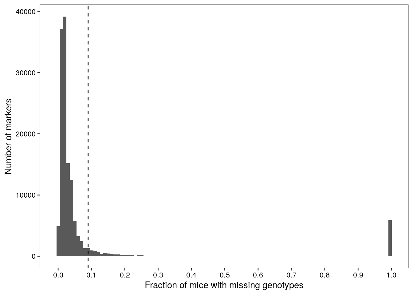
# Determine the 90th percentile of no call rates among all markers
cutoff <- quantile(no.calls$freq, probs = seq(0,1,0.05))[[19]]Of 137337 markers, 135944 failed to genotype at least one sample, and 13348 markers failed to genotype at least 9% of samples.
| Version | Author | Date |
|---|---|---|
| 3501596 | sam-widmayer | 2022-11-09 |
Sample QC
Searching for samples with poor marker representation
In a similar fashion, we calculated the number of reference samples with missing genotypes. Repeated observations of samples/strains with identical names meant that genotype counts for each marker among them couldn’t be grouped and tallied, so determining no-call frequency occurred column-wise. Mouse over individual samples to see the number of markers with missing genotypes for each sample.
# Determine the 95th percentile of no calls identified among all samples
bad_sample_cutoff <- quantile(n.calls.strains.df$n.no.calls, probs = seq(0,1,0.05))[20]

# Plot the number of no calls identified in each sample across all markers
sampleQC <- ggplot(n.calls.strains.df,
                   mapping = aes(x = reorder(sample_id,n.no.calls),
                                 y = n.no.calls,
                                 text = paste("Sample:", sample_id))) +
  geom_point() +
  QCtheme +
  theme(axis.text.x = element_blank(),
        axis.ticks.x = element_blank()) +
  geom_hline(yintercept = bad_sample_cutoff, linetype = 2) +
  labs(x = "Number of mice with missing genotypes",
       y = "Number of markers")
ggplotly(sampleQC, tooltip = c("text","y"))
Warning: `gather_()` was deprecated in tidyr 1.2.0.
ℹ Please use `gather()` instead.
ℹ The deprecated feature was likely used in the plotly package.
Please report the issue at <]8;;https://github.com/plotly/plotly.R/issueshttps://github.com/plotly/plotly.R/issues]8;;>.Validating sex of reference samples
We next validated the sexes of each sample using sex chromosome probe intensities. We paired up probe intensities, joined available metadata, and filtered down to only markers covering the X and Y chromosomes. Then we flagged markers with high missingness across all samples, as well as samples with high missingness among all markers.The first round of inferring predicted sexes used a rough search of the sample name for expected nomenclature convention, which includes a sex denotation.
## Tabulate the number of samples per predicted sex
predicted.sex.table <- predicted.sexes %>%
  dplyr::group_by(predicted.sex) %>%
  dplyr::count()
This captured 86 female samples, 130 male samples, leaving 63 samples of unknown predicted sex from nomenclature alone.
After predicting the sexes of the vast majority of reference samples, we visualized the average probe intensity among X Chromosome markers for each sample, labeling them by predicted sex. Samples colored black were unabled to have their sex inferred by the sample name, but cluster well with mice for which sex could be inferred. Conversely, some samples’ predicted sex is discordant with X and Y Chromosome marker intensities (i.e. blue samples that cluster with mostly orange samples, and vice versa). Mouse over individual dots to view the sample, as well as whether it was flagged for having many markers with missing genotype information. In many cases, pulling substrings of sample names as the sex of the sample was too sensitive and misclassified samples.
# Generate a plotting palette for each predicted sex (including unknown)
predicted.sex.plot.palettes <- sex.chr.intensities %>%
  dplyr::ungroup() %>%
  dplyr::distinct(sample_id, predicted.sex, high_missing_sample) %>%
  dplyr::mutate(predicted.sex.palette = dplyr::case_when(predicted.sex == "f" ~ "#5856b7",
                                                         predicted.sex == "m" ~ "#eeb868",
                                                         predicted.sex == "unknown" ~ "black"))
predicted.sex.palette <- predicted.sex.plot.palettes$predicted.sex.palette
names(predicted.sex.palette) <- predicted.sex.plot.palettes$predicted.sex

# Plot the Y Chromosome probe intensities against
# the sum of the average X and Y Chromosome probe intensities
mean.x.intensities.by.sex.plot <- sex.chr.intensities %>%
  dplyr::mutate(high_missing_sample = dplyr::if_else(high_missing_sample == "FLAG",
                                                     true = "Bad Samples",
                                                     false = "Good Samples")) %>%
  ggplot(., mapping = aes(x = mean.x.chr.int,
                         y = mean.y.int,
                         colour = predicted.sex,
                         text = sample_id)) +
  geom_point() +
  scale_colour_manual(values = predicted.sex.palette) +
  facet_grid(.~high_missing_sample) +
  QCtheme
ggplotly(mean.x.intensities.by.sex.plot,
         tooltip = c("text"))
Because the split between inferred sexes of good samples was so distinct for good samples, we used k-means clustering to quickly match the clusters to sexed samples and assign or re-assign sexes to samples with unknown or apparently incorrect sex information, respectively. Samples highlighted above were also re-evaluated using strain-specific marker information.
# Add a column to indicate whether a sample was reassigned a sex
# based on probe intensities
reSexed_samples_table <- reSexed_samples %>%
  dplyr::mutate(resexed = predicted.sex != inferred.sex)
reSexed_samples_table %>%
  dplyr::select(sample_id, resexed, predicted.sex, inferred.sex) %>%
  DT::datatable(., filter = "top",
              escape = FALSE)
The plot below demonstrates that this clustering technique does a pretty good job at capturing the information we want. Moving forward with sample QC we used the reassigned inferred sexes of the samples.
# Interactive scatter plot of intensities similar to above, but recolors
# and outlines samples based on redesignated sexes.
reSexed.plot <- ggplot(reSexed_samples_table %>%
                         dplyr::arrange(inferred.sex),
                       mapping = aes(x = mean.x.chr.int,
                                     y = mean.y.int,
                     fill = inferred.sex,
                     colour = predicted.sex,
                     text = sample_id,
                     label = resexed)) +
  geom_point(shape = 21,size = 3, alpha = 0.7) +
  scale_colour_manual(values =  predicted.sex.palette) +
  scale_fill_manual(values = predicted.sex.palette) +
  QCtheme
ggplotly(reSexed.plot,
         tooltip = c("text","label"))
Visualizing the corrected sex assignments, we can see two samples that stand out of the clusters: FAM and JAXMP_cookii_TH_BC19281. Because the X and Y probe intensities were supplied to k-means clustering independently in this datasest and the values for each channel were intermediate in this sample, FAM was predicted as female using the y channel and male using the x channel data. Because FAM is not a CC/DO founder or a sample representative of non-musculus species, we assigned this sample to the “unknown” sex category. JAXMP_cookii_TH_BC19281 clustered with both sexes in a similar fashion, but because of genetic divergence between its genome and the mouse reference genome from which probes were designed, the irregular probe intensity data is not unexpected. For this reason, and the Y channel data being much more consistent with female sample, we categorized this sample as female.
Validating reference sample genetic backgrounds
A key component of sample QC for our purposes is knowing that markers that we expect to deliver the consensus genotype (i.e. in a cross) actually provide us the correct strain information and allow us to correctly infer haplotypes.
# Display a table for all samples derived from CC/DO founders
# Dam names = row names; Sire name = column names
founder_sample_table <- founderSamples %>%
  dplyr::group_by(dam,sire) %>%
  dplyr::count() %>%
  tidyr::pivot_wider(names_from = sire, values_from = n)
DT::datatable(founder_sample_table, escape = FALSE,
              options = list(columnDefs = list(list(width = '20%',
                                                    targets = c(8)))))
From the table, we can see that all possible pairwise combinations of CC/DO founder strains are represented, with the exception of (NZO/HILtJxCAST/EiJ)F1 and (NZO/HILtJxPWK/PhJ)F1. These missing samples could be interesting; these two crosses have been previously noted as “reproductively incompatible” in the literature. We constructed a rough dendrogram from good marker genotypes to determine whether samples cluster according to known relationships among founder strains. Edge colors represent rough clustering into six groups - three of which contain samples derived from wild-derived founder strains and their F1 hybrids with other founder strains.
# File paths for wide reference genotypes in numerical genotype coding
# (output from GigaMUGA_FounderDendGenos.R)
recoded_wide_geno_files <- list.files("data/GigaMUGA/GigaMUGA_founder_sample_dendrogram_genos//",
                                      pattern = "gm_widegenos_chr")

# Read wide reference genotypes
recoded_wide_sample_genos_list <- list()
for(i in 1:length(recoded_wide_geno_files)){
  recoded_wide_sample_genos_list[[i]] <- fst::read.fst(
    path = paste0("data/GigaMUGA/GigaMUGA_founder_sample_dendrogram_genos/",
                  recoded_wide_geno_files[[i]]))
}
recoded_wide_sample_genos <- Reduce(dplyr::bind_cols,
                                    recoded_wide_sample_genos_list)

# Assign sample names as row names
sample_id_cols <- recoded_wide_sample_genos %>%
  dplyr::select(contains("sample_id"))
recoded_wide_sample_genos_nosamps <- recoded_wide_sample_genos %>%
  dplyr::select(-contains("sample_id"))
rownames(recoded_wide_sample_genos_nosamps) <- sample_id_cols[,1]

# Scale the genotype matrix, then calculate
# euclidean distance between all samples
dd <- dist(scale(recoded_wide_sample_genos_nosamps), method = "euclidean")
hc <- hclust(dd, method = "ward.D2")

# Plot sample distances as a dendrogram
dend_colors = c("slateblue",
                "blue",
                qtl2::CCcolors[6:8])
clus8 = cutree(hc, 5)
plot(as.phylo(hc), type = "f", cex = 0.5, tip.color = dend_colors[clus8],
     no.margin = T, label.offset = 1, edge.width = 0.5)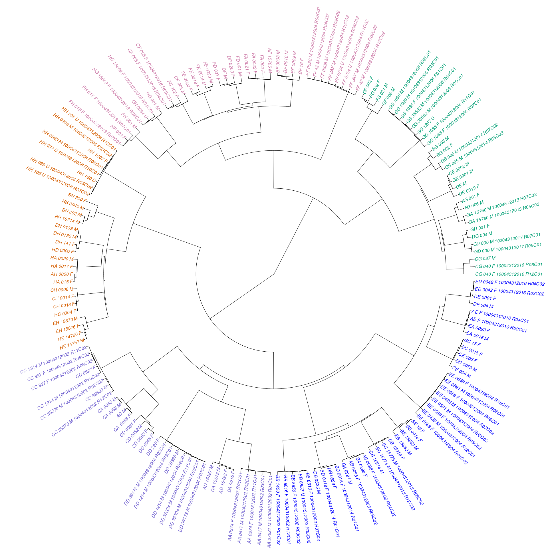
| Version | Author | Date |
|---|---|---|
| 3501596 | sam-widmayer | 2022-11-09 |
From here we curated a set of consensus genotypes for each CC/DO founder strain by identifying alleles that were fixed across replicate samples from each founder strain. Where there were discrepancies or missing genotypes among these samples, we used reconstructed haplotypes from over 950 DO mice to impute the genotypes for these sites. The consensus genotypes for intersecting markers between two founder strains were combined (“crossed”) to form predicted genotypes for each F1 hybrid of CC/DO founders. Then, the genotypes of each CC/DO founder F1 hybrid were compared directly to what was predicted, and the concordance shown below is the proportion of markers of each individual that match this prediction.
# Concordance file paths
# (output from GigaMUGA_ConsensusGenos.R)
chr_concordance_files <- list.files("data/GigaMUGA/GigaMUGA_founder_sample_concordance/")

# Read in concordance results from each chromosome and combine into a df
chr_concordance_list <- list()
for(i in 1:length(chr_concordance_files)){
  chr_concordance_list[[i]] <- fst::read.fst(path = paste0("data/GigaMUGA/GigaMUGA_founder_sample_concordance/",chr_concordance_files[[i]]))
}
founder_concordance_df <- Reduce(dplyr::full_join, chr_concordance_list)

# Join founder sample metadata and calculate concordance percentages
founder_concordance_df_3 <- founder_concordance_df %>%
  dplyr::left_join(., founderSamples %>%
                     dplyr::rename(sample = sample_id) %>%
                     dplyr::select(sample, dam, sire)) %>%
  dplyr::group_by(sample, alt_chr, dam, sire, inferred.sex) %>%
  dplyr::summarise(total.MATCH = sum(MATCH),
                   total.NO_MATCH = sum(`NO MATCH`),
                   concordance = total.MATCH/(total.MATCH+total.NO_MATCH))

# Subset into autosomal concordance metrics
auto_concordance <- founder_concordance_df_3 %>%
  dplyr::filter(alt_chr == "Autosome")

# Subset into Chromosome X concordance metrics
X_concordance <- founder_concordance_df_3 %>%
  dplyr::filter(alt_chr == "X")

# Plot autosomal concordance results interactively
founder_palette <- qtl2::CCcolors
names(founder_palette) <- unique(founderSamples$dam)
auto_concordance_plot <- ggplot(auto_concordance, mapping = aes(x = dam,
                                                          y = concordance,
                                                          color = dam,
                                                          fill = sire,
                                                          label = sample,
                                                          text = concordance)) +
  geom_jitter(shape = 21, width = 0.25) +
  scale_fill_manual(values = founder_palette) +
  scale_colour_manual(values = founder_palette) +
  labs(x = "Dam Founder Strain",
       y = "Autosomal Genotype Concordance") +
  facet_grid(.~inferred.sex) +
  QCtheme +
  theme(axis.text.x = element_text(angle = 45, hjust = 1, vjust = 1))
ggplotly(auto_concordance_plot, tooltip = c("label", "text"))
# Plot Chromosome X concordance results interactively
X_concordance_plot <- ggplot(X_concordance, mapping = aes(x = dam,
y = concordance,
color = dam,
fill = sire,
label = sample,
text = concordance)) +
geom_jitter(shape = 21, width = 0.25) +
scale_fill_manual(values = founder_palette) +
scale_colour_manual(values = founder_palette) +
labs(x = "Dam Founder Strain",
y = "X Chromosome Genotype Concordance") +
facet_grid(.~inferred.sex) +
QCtheme +
theme(axis.text.x = element_text(angle = 45, hjust = 1, vjust = 1))
ggplotly(X_concordance_plot, tooltip = c("label","text"))We identified one sample, GC_15_F which appears to be a strain mixup. Based on the sample name, the sample is predicted to be an F1 hybrid from a cross between a PWK/PhJ female and 129S1/SvImJ male. This sample, however does not group with any other PWK/PhJ-derived samples in our sample dendrogram and, instead, falls in with other NZO/HILtJ samples. Additionally, the strain concordance above indicates that both autosomes and the X chromosome are nearly 50% concordant. This led us to hypothesize that the sample was in fact an (NZO/HILtJx129S1/SvImJ)F1 mouse. We performed an additional check to test this and, as displayed below, we have good evidence that this was indeed the case. We have indicated this switch in all sample metadata files.
# Path to GC_15_F concordance results
GC_15_F_files <- list.files("data/GigaMUGA/GC_15_F_ReSex_Results/")

# Read in GC_15_F concordance results
GC_15_F_list <- list()
for(i in 1:length(GC_15_F_files)){
  GC_15_F_list[[i]] <- read.csv(file = paste0("data/GigaMUGA/GC_15_F_ReSex_Results/",GC_15_F_files[[i]])) %>%
    dplyr::mutate(chr = as.character(chr))
}
GC_15_F_concordance_df <- Reduce(dplyr::bind_rows, GC_15_F_list)
GC_15_F_concordance_df[is.na(GC_15_F_concordance_df)] <- 0

# Join sample metadata to GC_15_F concordance
GC_15_F_concordance_summary <- GC_15_F_concordance_df %>%
  dplyr::left_join(., founderSamples %>%
                     dplyr::rename(sample = sample_id) %>%
                     dplyr::select(sample, dam, sire)) %>%
  # Explicitly switch the dam genetic background
  dplyr::mutate(dam = "NZO/HILtJ") %>%
  dplyr::group_by(sample, alt_chr, dam, sire, inferred.sex) %>%
  # Calculate concordance
  dplyr::summarise(total.MATCH = sum(MATCH),
                   total.NO_MATCH = sum(NO.MATCH),
                   concordance = total.MATCH/(total.MATCH+total.NO_MATCH))

# Display data table of autosomal and Chr X concordance results
DT::datatable(GC_15_F_concordance_summary, escape = FALSE)
In the chunk below, all reference genotype files are prepared for writing.
# Filter out samples from non-musculus species from bad sample list
bad_samples <- high.n.samples %>%
  dplyr::filter(!sample_id %in% c("JAXMP_caroli_UNK_BC21325",
                                  "JAXMP_minu_KE_BC24327",
                                  "JAXMP_minu_KE_BC24339",
                                  "JAXMP_pahari_TH_BC21314"))

#############################################
## Write Reference Genotypes - All Samples ##
#############################################

# File paths for reference genotypes of each chromosome for CC/DO founder samples
founder_samp_genos_chr1_19 <- list.files(path = "data/GigaMUGA/GigaMUGA_founder_sample_genotypes/",
                                         pattern = "gm_founder_genos_chr_")[1:19]
founder_samp_genos_chrX <- list.files(path = "data/GigaMUGA/GigaMUGA_founder_sample_genotypes/",
                                          pattern ="gm_founder_genos_chr_")[20]
founder_sample_geno_files <- c(as.list(founder_samp_genos_chr1_19),"M","NA",founder_samp_genos_chrX,"Y")

# File paths for reference genotypes of each chromosome for all samples
nonfounder_sample_geno_files <- as.list(list.files(path = "data/GigaMUGA/GigaMUGA_reference_genotypes/",
                                                   pattern = "gm_genos_chr_"))

# Establish furrr parallelization plan
future::plan(multisession, workers = 16)
make_chunks <- furrr:::make_chunks
make_chunks(n_x = length(founder_sample_geno_files), n_workers = 16)
[[1]]
[1] 1 2
[[2]]
[1] 3
[[3]]
[1] 4 5
[[4]]
[1] 6
[[5]]
[1] 7
[[6]]
[1] 8 9
[[7]]
[1] 10
[[8]]
[1] 11
[[9]]
[1] 12 13
[[10]]
[1] 14
[[11]]
[1] 15 16
[[12]]
[1] 17
[[13]]
[1] 18
[[14]]
[1] 19 20
[[15]]
[1] 21
[[16]]
[1] 22 23# Read in and filter reference genotypes for each chromosome to good samples and markers
reference_genos_list <- furrr::future_map2(.x = founder_sample_geno_files,
.y = nonfounder_sample_geno_files,
.f = writeReferenceGenotypes,
.options = furrr_options(seed = TRUE)) %>%
purrr::discard(., is.character)[1] "NO REFERENCE GENOTYPES"# Make one df with all reference genotypes
reference_genos_df <- Reduce(dplyr::bind_rows, reference_genos_list)
# Join metadata to reference genotypes and use it to order markers by build 39
# genetic and physical position
reference_genos_df %<>%
dplyr::left_join(., gm_metadata %>%
dplyr::select(marker, chr, bp_mm10, cM_cox)) %>%
dplyr::arrange(bp_mm10, cM_cox) %>%
select(-chr, -cM_cox, -bp_mm10)
###############################################
## Write Reference Intensities - All Samples ##
###############################################
# Read in probe intensities for each chromosome for all reference samples
# Creates a list of two-element lists (x- and y-channel probe intensities)
reference_intensities_list <- furrr::future_map(.x = nonfounder_sample_geno_files,
.f = writeReferenceIntensities,
.options = furrr_options(seed = TRUE))[1] "NO REFERENCE INTENSITIES"# Transpose the list to create a two element list of 23 elements each
reference_intensities_list_tr <- purrr::transpose(reference_intensities_list)Warning: Element 21 must be length 2, not 1# Extract first element (x-channel intensities for each chr) and combine into a df
reference_X_intensities_df <- reference_intensities_list_tr[[1]] %>%
purrr::keep(., is.data.frame) %>%
Reduce(dplyr::bind_rows, .)
# Extract first element (y-channel intensities for each chr) and combine into a df
reference_Y_intensities_df <- reference_intensities_list_tr[[2]] %>%
purrr::keep(., is.data.frame) %>%
Reduce(dplyr::bind_rows, .)
# Join metadata to intensities and use it to order markers by build 39
# genetic and physical position
reference_X_intensities_df %<>%
dplyr::left_join(., gm_metadata %>%
dplyr::select(marker, chr, bp_mm10, cM_cox)) %>%
dplyr::arrange(bp_mm10, cM_cox) %>%
select(-chr, -cM_cox, -bp_mm10)
reference_Y_intensities_df %<>%
dplyr::left_join(., gm_metadata %>%
dplyr::select(marker, chr, bp_mm10, cM_cox)) %>%
dplyr::arrange(bp_mm10, cM_cox) %>%
select(-chr, -cM_cox, -bp_mm10)
#################################################
## Write Consensus Genotypes - Founder Strains ##
#################################################
# File paths for consensus genotypes of each chromosome for CC/DO founder strains
founder_consensus_files <- list.files(path = "data/GigaMUGA/GigaMUGA_founder_consensus_genotypes/",
pattern = "GigaMUGA_founder_consensus_imputed_genotypes_chr")
# Read in founder consensus genotypes and combine into one df
founder_consensus_genos <- purrr::map(.x = founder_consensus_files,
.f = writeFounderConsensusGenotypes) %>%
Reduce(dplyr::bind_rows, .)
# Convert consensus genotypes to single letter genotypes
# All genotypes homozygous from script that generates them
for(i in 2:ncol(founder_consensus_genos)){
founder_consensus_genos[,i] <- unlist(purrr::transpose(strsplit(founder_consensus_genos[,i],""))[[1]])
}
# Read in high-quality Y chromosome genotypes
founder_consensus_genos_Y <- read.csv(file = "output/GigaMUGA/GigaMUGA_founder_consensus_genotypes_chrY.csv") %>%
dplyr::select(-X) %>%
`colnames<-`(colnames(founder_consensus_genos))
# Read in high-quality Mt genotypes
founder_consensus_genos_M <- read.csv(file = "output/GigaMUGA/GigaMUGA_founder_consensus_genotypes_chrM.csv") %>%
dplyr::select(-X) %>%
`colnames<-`(colnames(founder_consensus_genos))
# Join Chr Y and Mt genotypes to the rest of the consensus genotypes
founder_consensus_genos %<>%
dplyr::bind_rows(., founder_consensus_genos_Y) %>%
dplyr::bind_rows(., founder_consensus_genos_M)
# Join with marker metadata, arrange by genetic and physical position
founder_consensus_genos %<>%
dplyr::left_join(., gm_metadata %>%
dplyr::select(marker, chr, bp_mm10, cM_cox)) %>%
dplyr::arrange(bp_mm10, cM_cox) %>%
select(-chr, -cM_cox, -bp_mm10)
# Change "-" calls to "N"
founder_consensus_genos[founder_consensus_genos == "-"] <- "N"
####################################
## Write Founder Mean Intensities ##
####################################
# Filter founder sample metadata to samples from founders (not F1s)
founder_samples_strains <- founderSamples %>%
dplyr::filter(bg == "INBRED") %>%
dplyr::distinct(sample_id, dam) %>%
dplyr::rename(strain = dam)
# Make x-channel intensities df long
founder_mean_x_ints <- reference_X_intensities_df %>%
dplyr::select(marker,founder_samples_strains$sample_id) %>%
tidyr::pivot_longer(-marker, names_to = "sample_id", values_to = "X") %>%
# Join founder sample metadata and remove null intensities
dplyr::left_join(., founder_samples_strains) %>%
dplyr::filter(!is.na(X)) %>%
# Calculate the average x-channel intensity for
# each marker among all of the same founder
dplyr::group_by(marker, strain) %>%
dplyr::summarise(mean_x = mean(X)) %>%
# Make df wide again
tidyr::pivot_wider(names_from = strain, values_from = mean_x) %>%
# Make sure that intensity file contains only markers from
# consensus file
dplyr::filter(marker %in% founder_consensus_genos$marker)
# Arrange x-channel intensity file by genetic and physical position
founder_mean_x_ints %<>%
dplyr::left_join(., gm_metadata %>%
dplyr::select(marker, chr, bp_mm10, cM_cox)) %>%
dplyr::arrange(bp_mm10, cM_cox) %>%
select(-chr, -cM_cox, -bp_mm10)
# Same process as x-channel intensities for y-channel intensities
founder_mean_y_ints <- reference_Y_intensities_df %>%
dplyr::select(marker,founder_samples_strains$sample_id) %>%
tidyr::pivot_longer(-marker, names_to = "sample_id", values_to = "Y") %>%
dplyr::left_join(., founder_samples_strains) %>%
dplyr::filter(!is.na(Y)) %>%
dplyr::group_by(marker, strain) %>%
dplyr::summarise(mean_y = mean(Y)) %>%
tidyr::pivot_wider(names_from = strain, values_from = mean_y) %>%
dplyr::filter(marker %in% founder_consensus_genos$marker)
founder_mean_y_ints %<>%
dplyr::left_join(., gm_metadata %>%
dplyr::select(marker, chr, bp_mm10, cM_cox)) %>%
dplyr::arrange(bp_mm10, cM_cox) %>%
select(-chr, -cM_cox, -bp_mm10)
###################################
## Write Founder Sample Metadata ##
###################################
# Wrangle founder metadata into final format
founder_metadata <- founderSamples %>%
dplyr::select(-bg) %>%
# Use different column names
dplyr::rename(original_sex = predicted.sex,
correct_sex = inferred.sex,
sample = sample_id) %>%
# Use correct F1 designation
dplyr::mutate(strain = dplyr::if_else(dam != sire,
true = paste0("(",dam,"x",sire,")F1"),
false = dam)) %>%
# Name strains using official nomenclature
dplyr::mutate(dam = case_when(dam == "A/J" ~ "A",
dam == "C57BL/6J" ~ "B",
dam == "129S1/SvImJ" ~ "C",
dam == "NOD/ShiLtJ" ~ "D",
dam == "NZO/HILtJ" ~ "E",
dam == "CAST/EiJ" ~ "F",
dam == "PWK/PhJ" ~ "G",
dam == "WSB/EiJ" ~ "H"),
sire = case_when(sire == "A/J" ~ "A",
sire == "C57BL/6J" ~ "B",
sire == "129S1/SvImJ" ~ "C",
sire == "NOD/ShiLtJ" ~ "D",
sire == "NZO/HILtJ" ~ "E",
sire == "CAST/EiJ" ~ "F",
sire == "PWK/PhJ" ~ "G",
sire == "WSB/EiJ" ~ "H")) %>%
# Make letter codes
tidyr::unite("letter", dam:sire, sep = "") %>%
dplyr::ungroup() %>%
dplyr::select(sample, strain, correct_sex, original_sex, letter) %>%
# Individual sample switch
dplyr::mutate(strain = if_else(sample == "GC_15_F",
true = "(NZO/HILtJx129S1/SvImJ)F1",
false = strain),
letter = if_else(sample == "GC_15_F",
true = "EC",
false = letter))
# Assemble metadata
reference_meta_nostrain <- predicted.sexes %>%
# Use samples present in the final reference genotype file
dplyr::filter(sample_id %in% colnames(reference_genos_df)[-1]) %>%
# Join sex check and smaple information
dplyr::left_join(., reSexed_samples %>%
dplyr::select(sample_id, inferred.sex)) %>%
dplyr::rename(sample = sample_id,
original_sex = predicted.sex,
correct_sex = inferred.sex) %>%
dplyr::left_join(., founder_metadata %>%
dplyr::select(sample, strain)) %>%
dplyr::mutate(strain = if_else(sample == "GC_15_F",
true = "(NZO/HILtJx129S1/SvImJ)F1",
false = strain))
# Idenfity strain names without strain information
unassigned_strains <- reference_meta_nostrain %>%
dplyr::filter(is.na(strain))
# Use regex searching to identify missing strains
new_strains <- purrr::map(unassigned_strains$sample, findStrain) %>%
unlist()
unassigned_strains$strain <- new_strains
reference_sample_metadata <- unassigned_strains %>%
dplyr::mutate(correct_sex = dplyr::if_else(is.na(correct_sex),
true = "unknown",
false = correct_sex),
mouse.id.1 = stringr::str_sub(strain, -1),
strain = dplyr::if_else(mouse.id.1 %in% c("m","f"),
true = str_sub(string = strain, 1, nchar(strain)-1),
false = strain)) %>%
dplyr::select(-mouse.id.1) %>%
dplyr::mutate(strain = dplyr::case_when(strain == "JAXMP_do" ~ "JAXMP_dom",
strain == "JAXMP_" ~ "JAXMP_minu",
strain == "PANCEVO/EiJ31581" ~ "PANCEVO/EiJ",
str_detect(string = strain, pattern = "MWN") ~ "MWN",
str_detect(string = strain, pattern = "PAE") ~ "PAE",
str_detect(string = strain, pattern = "JAXMP_pahari") ~ "JAXMP_pahari",
str_detect(string = strain, pattern = "JAXMP_spt") ~ "JAXMP_spt",
str_detect(string = strain, pattern = "JAXMP_cooki") ~ "JAXMP_cooki",
str_detect(string = strain, pattern = "JAXMP_cptak") ~ "JAXMP_cptak",
str_detect(string = strain, pattern = "JAXMP_caroli") ~ "JAXMP_caroli",
str_detect(string = strain, pattern = "JAXMP_hort") ~ "JAXMP_hort",
# A few remaining founder samples, not included in founder-specific
# analyses
str_detect(string = strain, pattern = "AA") ~ "A/J",
str_detect(string = strain, pattern = "BB") ~ "C57BL/6J",
TRUE ~ strain)) %>%
dplyr::bind_rows(.,reference_meta_nostrain %>%
dplyr::filter(!sample %in% unassigned_strains$sample)) %>%
dplyr::filter(sample %in% colnames(reference_genos_df)[-1]) %>%
dplyr::mutate(correct_sex = dplyr::case_when(sample == "FAM" ~ "unknown",
sample == "JAXMP_cookii_TH_BC19281" ~ "female",
TRUE ~ correct_sex)) %>%
dplyr::ungroup() %>%
dplyr::distinct()In addition, we identified 13 high-quality consensus genotypes on Chromosome Y and 20 genotypes on the mitochondria. We constructed dendrograms from both of these marker sets to estimate how many different Y haplogroups and mitotypes segregate among the CC/DO founders.
# Recode Chr Y consensus genotypes
founder_consensus_genos_Y_recoded <- suppressWarnings(data.frame(apply(founder_consensus_genos_Y[,2:ncol(founder_consensus_genos_Y)], 2, recodeCalls)))
founder_consensus_genos_Y_recoded %<>%
  dplyr::mutate(marker = founder_consensus_genos_Y$marker) %>%
  dplyr::select(marker, everything())
colnames(founder_consensus_genos_Y_recoded) <- colnames(founder_consensus_genos_Y)


# Scale the Y genotype matrix, then calculate
# euclidean distance between all samples
dd_Y <- dist(scale(t(founder_consensus_genos_Y_recoded[,-1])), method = "euclidean")
hc_Y <- hclust(dd_Y, method = "ward.D2")
plot(as.phylo(hc_Y),
     type = "u",
     cex = 1.5,
     tip.color = qtl2::CCcolors,
     no.margin = T, label.offset = 0.75, edge.width = 1)
From the dendrogram above, there appear to be six rough Y chromosome haplogroups segregating among the founders, as was previously reported.
# View six Chr Y clusters
six <- cutree(hc_Y, 6)
print(paste("Cluster 1: ", paste(names(six[which(six == 1)]), collapse = ", ")))
[1] "Cluster 1: A/J"print(paste("Cluster 2: ", paste(names(six[which(six == 2)]), collapse = ", ")))[1] "Cluster 2: C57BL/6J, 129S1/SvImJ, NZO/HILtJ"print(paste("Cluster 3: ", paste(names(six[which(six == 3)]), collapse = ", ")))[1] "Cluster 3: NOD/ShiLtJ"print(paste("Cluster 4: ", paste(names(six[which(six == 4)]), collapse = ", ")))[1] "Cluster 4: CAST/EiJ"print(paste("Cluster 5: ", paste(names(six[which(six == 5)]), collapse = ", ")))[1] "Cluster 5: PWK/PhJ"print(paste("Cluster 6: ", paste(names(six[which(six == 6)]), collapse = ", ")))[1] "Cluster 6: WSB/EiJ"# Make a data frame with just haplogroup 2
BCE <- founder_consensus_genos_Y[,c(1,which(colnames(founder_consensus_genos_Y) %in% names(six[which(six == 2)])))]
# If there is no variation within the haplogroup, condense the founders into one haplogroup
if(unique(apply(BCE[,2:4],1,function(x) length(unique(x)))) == 1){
BCE <- BCE[,1:2]
colnames(BCE)[2] <- "BCE"
}
y_haplos <- BCE %>% dplyr::left_join(., founder_consensus_genos_Y)
y_haplos %<>%
dplyr::select(marker, `A/J`, BCE, `NOD/ShiLtJ`, `CAST/EiJ`, `PWK/PhJ`, `WSB/EiJ`) %>%
`colnames<-`(c("marker", "A", "BCE", "D", "F", "G", "H"))We performed the same analysis using the mitochondrial markers.
# Recode Mt consensus genotypes
founder_consensus_genos_M_recoded <- suppressWarnings(data.frame(apply(founder_consensus_genos_M[,2:ncol(founder_consensus_genos_M)], 2, recodeCalls)))
founder_consensus_genos_M_recoded %<>%
  dplyr::mutate(marker = founder_consensus_genos_M$marker) %>%
  dplyr::select(marker, everything())
colnames(founder_consensus_genos_M_recoded) <- colnames(founder_consensus_genos_M)

# Scale the Mt genotype matrix, then calculate
# euclidean distance between all samples
dd_M <- dist(scale(t(founder_consensus_genos_M_recoded[,-1])), method = "euclidean")
hc_M <- hclust(dd_M, method = "ward.D2")
plot(as.phylo(hc_M),
     type = "u",
     cex = 1.5,
     tip.color = qtl2::CCcolors,
     no.margin = T, label.offset = 0, edge.width = 1)
From the above dendrogram, there are four clear haplogroups:
# View four mitochondrial clusters
four <- cutree(hc_M, 4)
print(paste("Cluster 1: ", paste(names(four[which(four == 1)]), collapse = ", ")))
[1] "Cluster 1: A/J, C57BL/6J, 129S1/SvImJ, NOD/ShiLtJ"print(paste("Cluster 2: ", paste(names(four[which(four == 2)]), collapse = ", ")))[1] "Cluster 2: NZO/HILtJ"print(paste("Cluster 3: ", paste(names(four[which(four == 3)]), collapse = ", ")))[1] "Cluster 3: CAST/EiJ, PWK/PhJ"print(paste("Cluster 4: ", paste(names(four[which(four == 4)]), collapse = ", ")))[1] "Cluster 4: WSB/EiJ"These results, In contrast to previously reports, demonstrate that PWK/PhJ and CAST/EiJ cluster together using these markers. However, when enforcing a five-cluster split, the PWK/PhJ and CAST/EiJ haplogroups split before any other cluster.
# View five mitochondrial clusters
five <- cutree(hc_M, 5)
print(paste("Cluster 1: ", paste(names(five[which(five == 1)]), collapse = ", ")))
[1] "Cluster 1: A/J, C57BL/6J, 129S1/SvImJ, NOD/ShiLtJ"print(paste("Cluster 2: ", paste(names(five[which(five == 2)]), collapse = ", ")))[1] "Cluster 2: NZO/HILtJ"print(paste("Cluster 3: ", paste(names(five[which(five == 3)]), collapse = ", ")))[1] "Cluster 3: CAST/EiJ"print(paste("Cluster 4: ", paste(names(five[which(five == 4)]), collapse = ", ")))[1] "Cluster 4: PWK/PhJ"print(paste("Cluster 5: ", paste(names(five[which(five == 4)]), collapse = ", ")))[1] "Cluster 5: PWK/PhJ"Additionally, five markers distinguish the two haplogroups.
# How many markers distinguish CAST and PWK mitochondrial haplogroups?
founder_consensus_genos_M %>%
  dplyr::select(marker, `CAST/EiJ`,`PWK/PhJ`) %>%
  dplyr::filter(`CAST/EiJ` != `PWK/PhJ`)
marker CAST/EiJ PWK/PhJ
1 Mit006 C T
2 Mit007 C T
3 Mit012 C T
4 Mit027 G A
5 Mit029 T C# Make a data frame with just haplogroup 2
ABCD <- founder_consensus_genos_M[,c(1,which(colnames(founder_consensus_genos_M) %in% names(five[which(five == 1)])))]
# If there is no variation within the haplogroup, condense the founders into one haplogroup
if(unique(apply(ABCD[,2:5],1,function(x) length(unique(x)))) == 1){
ABCD <- ABCD[,1:2]
colnames(ABCD)[2] <- "ABCD"
}
m_haplos <- ABCD %>% dplyr::left_join(., founder_consensus_genos_M)
m_haplos %<>%
dplyr::select(marker, ABCD, `NZO/HILtJ`, `CAST/EiJ`, `PWK/PhJ`, `WSB/EiJ`) %>%
`colnames<-`(c("marker", "ABCD", "E", "F", "G", "H"))Given that the five haplogroups separate the wild-derived founders from each subspecies, we recommend that this haplogroup structure be adopted for future haplotype reconstruction for the mitochondria in the DO for QTL mapping applications.
Writing reference files
The list of output file types following QC is as follows:
Genotype file; rows = markers, columns = samples
Probe intensity file; rows = markers, columns = samples
Sample metadata; columns = sample, strain, sex
Each file type is generated for:
All good samples
Eight CC/DO founder strains
###################
## WRITING FILES ##
###################

# Write reference genotypes
dir.create("output/GigaMUGA")
Warning in dir.create("output/GigaMUGA"): 'output/GigaMUGA' already existswrite.csv(reference_genos_df,
file = "output/GigaMUGA/GigaMUGA_genotypes.csv",
row.names = F)
if(file.exists("output/GigaMUGA/GigaMUGA_genotypes.csv.gz")){
system("rm output/GigaMUGA/GigaMUGA_genotypes.csv.gz")
}
system("gzip output/GigaMUGA/GigaMUGA_genotypes.csv")
# Write reference x-channel intensities
write.csv(reference_X_intensities_df,
file = "output/GigaMUGA/GigaMUGA_x_intensities.csv",
row.names = F)
if(file.exists("output/GigaMUGA/GigaMUGA_x_intensities.csv.gz")){
system("rm output/GigaMUGA/GigaMUGA_x_intensities.csv.gz")
}
system("gzip output/GigaMUGA/GigaMUGA_x_intensities.csv")
# Write reference y-channel intensities
write.csv(reference_Y_intensities_df,
file = "output/GigaMUGA/GigaMUGA_y_intensities.csv",
row.names = F)
if(file.exists("output/GigaMUGA/GigaMUGA_y_intensities.csv.gz")){
system("rm output/GigaMUGA/GigaMUGA_y_intensities.csv.gz")
}
system("gzip output/GigaMUGA/GigaMUGA_y_intensities.csv")
# Write sample metadata for all reference samples
write.csv(reference_sample_metadata,
file = "output/GigaMUGA/GigaMUGA_sample_metadata.csv",
row.names = F)
# Write founder consensus genotypes
write.csv(founder_consensus_genos,
file = "output/GigaMUGA/GigaMUGA_founder_consensus_genotypes.csv",
row.names = F)
if(file.exists("output/GigaMUGA/GigaMUGA_founder_consensus_genotypes.csv.gz")){
system("rm output/GigaMUGA/GigaMUGA_founder_consensus_genotypes.csv.gz")
}
system("gzip output/GigaMUGA/GigaMUGA_founder_consensus_genotypes.csv")
write.csv(m_haplos,
file = "output/GigaMUGA/GigaMUGA_founder_consensus_genotypes_Mt.csv",
row.names = F)
write.csv(y_haplos,
file = "output/GigaMUGA/GigaMUGA_founder_consensus_genotypes_Y.csv",
row.names = F)
# Write founder strain-averaged x-channel intensities
write.csv(founder_mean_x_ints,
file = "output/GigaMUGA/GigaMUGA_founder_mean_x_intensities.csv",
row.names = F)
if(file.exists("output/GigaMUGA/GigaMUGA_founder_mean_x_intensities.csv.gz")){
system("rm output/GigaMUGA/GigaMUGA_founder_mean_x_intensities.csv.gz")
}
system("gzip output/GigaMUGA/GigaMUGA_founder_mean_x_intensities.csv")
# Write founder strain-averaged y-channel intensities
write.csv(founder_mean_y_ints,
file = "output/GigaMUGA/GigaMUGA_founder_mean_y_intensities.csv",
row.names = F)
if(file.exists("output/GigaMUGA/GigaMUGA_founder_mean_y_intensities.csv.gz")){
system("rm output/GigaMUGA/GigaMUGA_founder_mean_y_intensities.csv.gz")
}
system("gzip output/GigaMUGA/GigaMUGA_founder_mean_y_intensities.csv")
# Write founder sample metadata
write.csv(founder_metadata,
file = "output/GigaMUGA/GigaMUGA_founder_metadata.csv",
row.names = F)
sessionInfo()R version 4.2.1 (2022-06-23)
Platform: x86_64-pc-linux-gnu (64-bit)
Running under: Ubuntu 20.04.5 LTS
Matrix products: default
BLAS: /usr/lib/x86_64-linux-gnu/openblas-pthread/libblas.so.3
LAPACK: /usr/lib/x86_64-linux-gnu/openblas-pthread/liblapack.so.3
locale:
[1] LC_CTYPE=en_US.UTF-8 LC_NUMERIC=C
[3] LC_TIME=en_US.UTF-8 LC_COLLATE=en_US.UTF-8
[5] LC_MONETARY=en_US.UTF-8 LC_MESSAGES=en_US.UTF-8
[7] LC_PAPER=en_US.UTF-8 LC_NAME=C
[9] LC_ADDRESS=C LC_TELEPHONE=C
[11] LC_MEASUREMENT=en_US.UTF-8 LC_IDENTIFICATION=C
attached base packages:
[1] parallel stats graphics grDevices utils datasets methods
[8] base
other attached packages:
[1] fstcore_0.9.12 vroom_1.6.0 tictoc_1.1 RColorBrewer_1.1-3
[5] ape_5.6-2 progress_1.2.2 plotly_4.10.0 ggplot2_3.3.6
[9] DT_0.26 magrittr_2.0.3 qtl2_0.28 furrr_0.3.1
[13] future_1.28.0 purrr_0.3.5 data.table_1.14.4 stringr_1.4.1
[17] tidyr_1.2.1 dplyr_1.0.10 fst_0.9.8
loaded via a namespace (and not attached):
[1] httr_1.4.4 sass_0.4.2 bit64_4.0.5 jsonlite_1.8.3
[5] viridisLite_0.4.1 bslib_0.4.0 assertthat_0.2.1 highr_0.9
[9] blob_1.2.3 yaml_2.3.6 globals_0.16.1 pillar_1.8.1
[13] RSQLite_2.2.18 lattice_0.20-45 glue_1.6.2 digest_0.6.30
[17] promises_1.2.0.1 colorspace_2.0-3 htmltools_0.5.3 httpuv_1.6.6
[21] pkgconfig_2.0.3 listenv_0.8.0 scales_1.2.1 whisker_0.4
[25] later_1.3.0 tzdb_0.3.0 git2r_0.30.1 tibble_3.1.8
[29] farver_2.1.1 generics_0.1.3 ellipsis_0.3.2 cachem_1.0.6
[33] withr_2.5.0 lazyeval_0.2.2 cli_3.4.1 crayon_1.5.2
[37] memoise_2.0.1 evaluate_0.17 fs_1.5.2 fansi_1.0.3
[41] parallelly_1.32.1 nlme_3.1-157 tools_4.2.1 prettyunits_1.1.1
[45] hms_1.1.2 lifecycle_1.0.3 munsell_0.5.0 compiler_4.2.1
[49] jquerylib_0.1.4 rlang_1.0.6 grid_4.2.1 rstudioapi_0.14
[53] htmlwidgets_1.5.4 crosstalk_1.2.0 labeling_0.4.2 rmarkdown_2.17
[57] gtable_0.3.1 codetools_0.2-18 DBI_1.1.3 R6_2.5.1
[61] knitr_1.40 fastmap_1.1.0 bit_4.0.4 utf8_1.2.2
[65] workflowr_1.7.0 rprojroot_2.0.3 stringi_1.7.8 Rcpp_1.0.9
[69] vctrs_0.5.0 tidyselect_1.2.0 xfun_0.34