Reference Data QC: MUGA
Last updated: 2023-01-13
Checks: 7 0
Knit directory: MUGA_reference_data/
This reproducible R Markdown analysis was created with workflowr (version 1.7.0). The Checks tab describes the reproducibility checks that were applied when the results were created. The Past versions tab lists the development history.
Great! Since the R Markdown file has been committed to the Git repository, you know the exact version of the code that produced these results.
Great job! The global environment was empty. Objects defined in the global environment can affect the analysis in your R Markdown file in unknown ways. For reproduciblity it’s best to always run the code in an empty environment.
The command set.seed(20221108) was run prior to running
the code in the R Markdown file. Setting a seed ensures that any results
that rely on randomness, e.g. subsampling or permutations, are
reproducible.
Great job! Recording the operating system, R version, and package versions is critical for reproducibility.
Nice! There were no cached chunks for this analysis, so you can be confident that you successfully produced the results during this run.
Great job! Using relative paths to the files within your workflowr project makes it easier to run your code on other machines.
Great! You are using Git for version control. Tracking code development and connecting the code version to the results is critical for reproducibility.
The results in this page were generated with repository version 83baed5. See the Past versions tab to see a history of the changes made to the R Markdown and HTML files.
Note that you need to be careful to ensure that all relevant files for
the analysis have been committed to Git prior to generating the results
(you can use wflow_publish or
wflow_git_commit). workflowr only checks the R Markdown
file, but you know if there are other scripts or data files that it
depends on. Below is the status of the Git repository when the results
were generated:
Ignored files:
    Ignored:    .DS_Store
    Ignored:    .Rhistory
    Ignored:    .Rproj.user/
    Ignored:    code/.DS_Store
    Ignored:    data/.DS_Store
    Ignored:    output/.DS_Store
    Ignored:    output/MUGA/.DS_Store

Untracked files:
    Untracked:  README.html
    Untracked:  code/README.html
    Untracked:  data/GigaMUGA/FPGM_1-6_FinalReport.txt
    Untracked:  data/GigaMUGA/FPGM_1-6_FinalReport.zip
    Untracked:  data/GigaMUGA/GC_15_F_ReSex_Results/
    Untracked:  data/GigaMUGA/GigaMUGA_control_genotypes.txt
    Untracked:  data/GigaMUGA/GigaMUGA_founder_consensus_genotypes/
    Untracked:  data/GigaMUGA/GigaMUGA_founder_sample_concordance/
    Untracked:  data/GigaMUGA/GigaMUGA_founder_sample_dendrogram_genos/
    Untracked:  data/GigaMUGA/GigaMUGA_founder_sample_genotypes/
    Untracked:  data/GigaMUGA/GigaMUGA_reference_genotypes/
    Untracked:  output/GigaMUGA/

Unstaged changes:
    Deleted:    code/workflowr_build.R
    Modified:   output/MUGA/MUGA_founder_consensus_genotypes.csv.gz
    Modified:   output/MUGA/MUGA_founder_mean_x_intensities.csv.gz
    Modified:   output/MUGA/MUGA_founder_mean_y_intensities.csv.gz
    Modified:   output/MUGA/MUGA_founder_metadata.csv
    Modified:   output/MUGA/MUGA_genotypes.csv.gz
    Modified:   output/MUGA/MUGA_sample_metadata.csv
    Modified:   output/MUGA/MUGA_x_intensities.csv.gz
    Modified:   output/MUGA/MUGA_y_intensities.csv.gz
    Deleted:    output/MegaMUGA/MegaMUGA_founder_consensus_genotypes.csv.gz
    Deleted:    output/MegaMUGA/MegaMUGA_founder_mean_x_intensities.csv.gz
    Deleted:    output/MegaMUGA/MegaMUGA_founder_mean_y_intensities.csv.gz
    Deleted:    output/MegaMUGA/MegaMUGA_founder_metadata.csv
    Deleted:    output/MegaMUGA/MegaMUGA_genotypes.csv.gz
    Deleted:    output/MegaMUGA/MegaMUGA_sample_metadata.csv
    Deleted:    output/MegaMUGA/MegaMUGA_x_intensities.csv.gz
    Deleted:    output/MegaMUGA/MegaMUGA_y_intensities.csv.gz
Note that any generated files, e.g. HTML, png, CSS, etc., are not included in this status report because it is ok for generated content to have uncommitted changes.
These are the previous versions of the repository in which changes were
made to the R Markdown (analysis/MUGA_Reference_QC.Rmd) and
HTML (docs/MUGA_Reference_QC.html) files. If you’ve
configured a remote Git repository (see ?wflow_git_remote),
click on the hyperlinks in the table below to view the files as they
were in that past version.
| File | Version | Author | Date | Message |
|---|---|---|---|---|
| Rmd | 877e958 | sam-widmayer | 2023-01-13 | ref data changes for GEDI link |
| html | 49493e0 | sam-widmayer | 2022-11-18 | Build site. |
| Rmd | 05c642f | sam-widmayer | 2022-11-18 | wflow_publish("analysis/MUGA_Reference_QC.Rmd") |
| html | 025f6f8 | sam-widmayer | 2022-11-09 | Build site. |
| Rmd | d352284 | sam-widmayer | 2022-11-09 | update site theme and fold code snippets |
| html | d352284 | sam-widmayer | 2022-11-09 | update site theme and fold code snippets |
| Rmd | 3501596 | sam-widmayer | 2022-11-09 | change site theme and add index tables |
| html | 3501596 | sam-widmayer | 2022-11-09 | change site theme and add index tables |
| Rmd | 1074529 | sam-widmayer | 2022-11-08 | update markdown formatting for workflowr |
| Rmd | efe8849 | sam-widmayer | 2022-11-08 | initialize workflowr integration |
MUGA Annotations
Reading in reference genotypes and metadata
First I read in the reference sample genotypes, as well as marker annotations from an analysis previously conducted by Karl Broman, Dan Gatti, and Belinda Cornes.
## Reading in marker annotations fro Broman, Gatti, & Cornes analysis
pre_control_genotypes <- data.table::fread("data/MUGA/vendu.dodata.csv", header = T)
samples <- unique(colnames(pre_control_genotypes)[-c(1:3)])
control_genotypes <- data.table::fread("data/MUGA/vendu.dodata.csv", header = T, skip = 1)

tidy_control_genotypes <- purrr::map(samples, tidyMUGAgenos) %>%
  Reduce(rbind,.) %>%
  dplyr::rename(marker = snpID,
                genotype = call)
muga_metadata <- data.table::fread("data/MUGA/muga_uwisc_v2.csv", header = T)
Marker QC: Searching for missing genotype calls
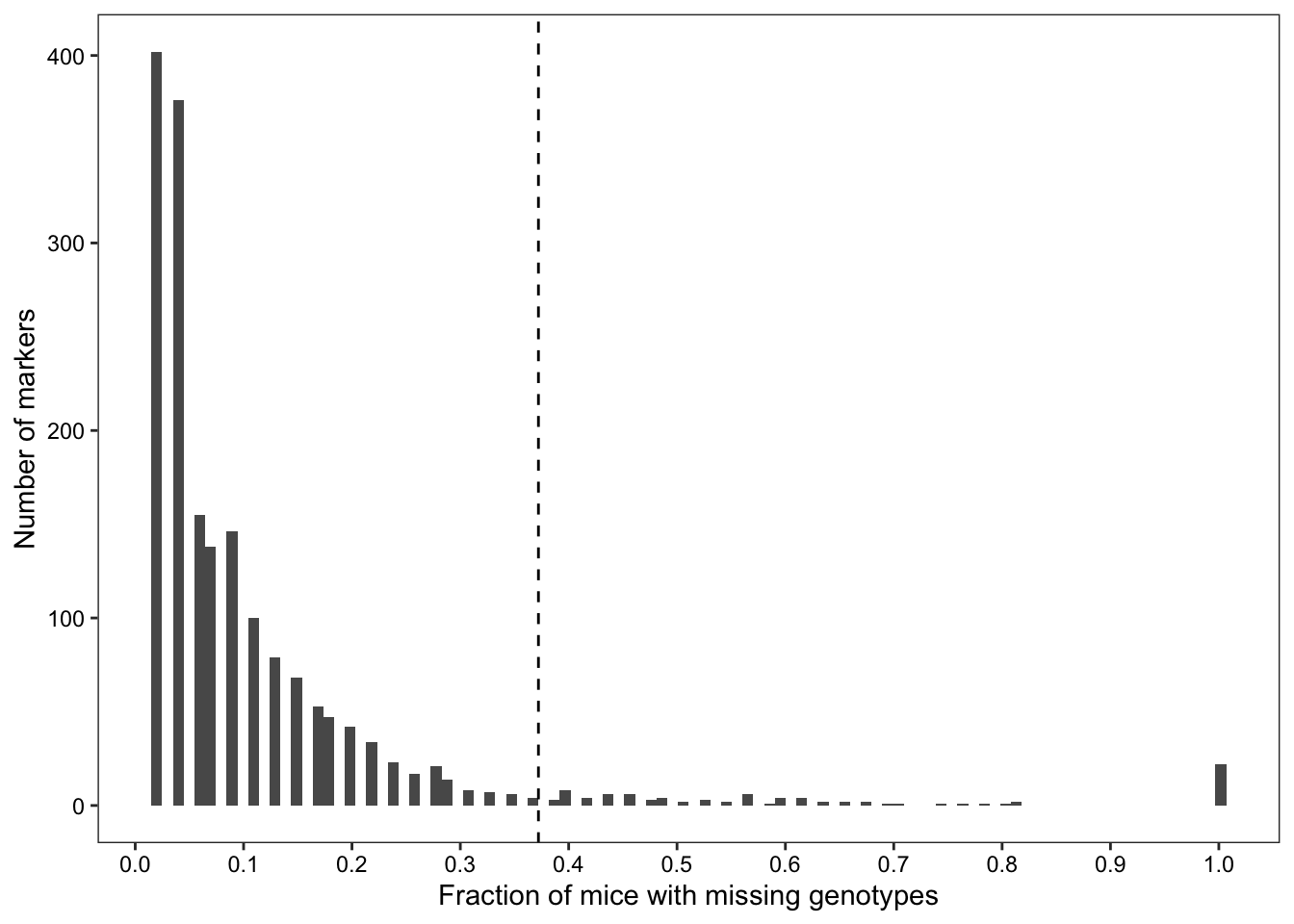
We searched for probes where many mice are missing genotype calls.
## Calculating allele frequencies for each marker
control_allele_freqs <- tidy_control_genotypes %>%
  dplyr::select(sample, marker, genotype) %>%
  dplyr::group_by(marker, genotype) %>%
  dplyr::count() %>%
  # Result: number of genotype calls for each marker across all samples
  # i.e.
#    marker            genotype     n
#    <chr>             <chr>    <int>
#  1 backupJAX00000484 A           12
#  2 backupJAX00000484 G           21
#  3 backupJAX00000484 H           22
#  4 backupJAX00003592 A           14
#  5 backupJAX00003592 G           18
#  6 backupJAX00003592 H           23
#  7 backupJAX00004293 C           16
#  8 backupJAX00004293 H           24
#  9 backupJAX00004293 T           15
# 10 backupJAX00005508 A            8
  dplyr::ungroup() %>%
  dplyr::group_by(marker) %>%
  dplyr::mutate(freq = round(n/sum(n), 3),
                genotype = as.factor(genotype)) %>%
  # Result: allele frequency calls for each marker across all samples
  # i.e.
#    marker            genotype     n  freq
#    <chr>             <fct>    <int> <dbl>
#  1 backupJAX00000484 A           12 0.218
#  2 backupJAX00000484 G           21 0.382
#  3 backupJAX00000484 H           22 0.4
#  4 backupJAX00003592 A           14 0.255
#  5 backupJAX00003592 G           18 0.327
#  6 backupJAX00003592 H           23 0.418
#  7 backupJAX00004293 C           16 0.291
#  8 backupJAX00004293 H           24 0.436
#  9 backupJAX00004293 T           15 0.273
# 10 backupJAX00005508 A            8 0.145
  dplyr::left_join(., muga_metadata)


## Filtering to markers with missing genotypes
no.calls <- control_allele_freqs %>%
  dplyr::ungroup() %>%
  dplyr::filter(genotype == "N") %>%
  tidyr::pivot_wider(names_from = genotype,
                     values_from = n) %>%
  dplyr::select(marker, chr, bp_grcm39, freq) %>%
  dplyr::mutate(chr = as.factor(chr))


## Identifying markers with missing genotypes at a frequency higher than the 95th percentile of "N" frequencies across all markers
cutoff <- quantile(no.calls$freq, probs = seq(0,1,0.05))[[20]]
above.cutoff <- no.calls %>%
  dplyr::filter(freq > cutoff)
Of 7854 markers, 1832 failed to genotype at least one sample, and 92 markers failed to genotype at least 37.21% of samples.
| Version | Author | Date |
|---|---|---|
| 3501596 | sam-widmayer | 2022-11-09 |
Sample QC
Searching for samples with poor marker representation
We calculated the number of reference samples with missing genotypes. Mouse over individual samples to see the number of markers with missing genotypes for each sample.
## Calculating the number of missing markers for each sample
n.calls.strains.df <- tidy_control_genotypes %>%
  dplyr::select(sample, marker, genotype) %>%
  dplyr::group_by(sample, genotype) %>%
  dplyr::count() %>%
  dplyr::filter(genotype == "N") %>%
  dplyr::ungroup() %>%
  dplyr::select(sample, n) %>%
  dplyr::rename(n.no.calls = n)
#    sample              n.no.calls
#    <chr>                    <int>
#  1 #1-m-9376 (m)              149
#  2 #2-m-9376 (m)              201
#  3 #3-m-9376 (m)              191
#  4 #4-m-9376 (m)              226
#  5 #5-m-9376 (m)              217
#  6 #6-m-9376 (m)              154
#  7 129S1/SvImJ (f)            176
#  8 129S1/SvImJm212 (m)        158
#  9 129xCASTf005 (f)           113
# 10 129xPWK 040F (f)           108


## Interactive plot of the number of missing genotypes for each sample.
sampleQC <- ggplot(n.calls.strains.df,
                   mapping = aes(x = reorder(sample,n.no.calls),
                                 y = n.no.calls,
                                 text = paste("Sample:", sample))) +
  geom_point() +
  QCtheme +
  theme(axis.text.x = element_blank(),
        axis.ticks.x = element_blank()) +
  labs(x = "Number of mice with missing genotypes",
       y = "Number of markers")
ggplotly(sampleQC, tooltip = c("text","y"))
From the sample QC plot, we can see that one of the NOD/ShiLtJ references samples is missing 391 genotypes, reducing our confidence in its use for consensus building. We exclude this sample in subsequent analyses.
Validating sex of reference samples
We next validated the sexes of each sample using sex chromosome probe intensities. We paired up probe intensities, joined available metadata, and filtered down to only markers covering the X and Y chromosomes.
## Bad samples
bad_samples <- c("NOD/ShiLtJ-35335 (m)")

## Reading in genotype intensities
long_intensities <- tidy_control_genotypes %>%
  dplyr::select(sample, marker, Chromosome, Position, genotype, X, Y, theta)

## Joining intensity files with marker metadata and reducing to markers on sex chromosomes
long_XY_intensities <- long_intensities %>%
  dplyr::left_join(., muga_metadata) %>%
  dplyr::filter(Chromosome %in% c("X","Y"),
                !sample %in% bad_samples)

# Expected output
#                 sample       marker Chromosome Position genotype     X     Y theta  chr
#     1:   #1-m-9376 (m) UNC200279739          X  4324915        H 0.745 1.560 0.716 <NA>
#     2:   #1-m-9376 (m) UNC200000454          X  5080366        T 0.903 0.019 0.013    X
#     3:   #1-m-9376 (m) UNC200001507          X  5282192        H 1.791 1.417 0.426 <NA>
#     4:   #1-m-9376 (m) UNC200282646          X  5667495        A 0.446 0.010 0.014    X
#     5:   #1-m-9376 (m) UNC200880603          X  5938298        G 0.016 0.517  0.98    X
#    ---
# 26996: WSBxPWKf003 (f) UNC210001275          Y    38376        N 0.028 0.030  0.52    Y
# 26997: WSBxPWKf003 (f) UNC210000095          Y   415819        T 1.710 0.808 0.281    Y
# 26998: WSBxPWKf003 (f) UNC210001366          Y   987513        A 2.216 0.378 0.108    Y
# 26999: WSBxPWKf003 (f) UNC210000599          Y  1246957        H 0.039 0.056  0.61    Y
# 27000: WSBxPWKf003 (f) UNC210001613          Y  2638355        G 0.020 1.339  0.99    Y
#        bp_mm10 bp_grcm39   cM_cox strand snp unique unmapped
#     1:      NA        NA       NA   <NA>  AG  FALSE    FALSE
#     2: 5503248   5415302 1.131211  minus  AC   TRUE    FALSE
#     3:      NA        NA       NA   <NA>  AG  FALSE    FALSE
#     4: 6090377   6002431 1.406192   plus  AG   TRUE    FALSE
#     5: 6361180   6273234 1.533023  minus  TC   TRUE    FALSE
#    ---
# 26996:  701933    701933       NA  minus  TC   TRUE    FALSE
# 26997: 1079376   1079376       NA  minus  AG   TRUE    FALSE
# 26998: 1731565   1731565       NA  minus  TG   TRUE    FALSE
# 26999: 1991009   1991009       NA   plus  AG   TRUE    FALSE
# 27000: 4022770   4022770       NA   plus  AG   TRUE    FALSE
#                                                     probe strand_flipped
#     1: ATTCTTTGAATTTGTTCAGTGTCTCTTGTTAGGACTGTACTTTCATTTCT          FALSE
#     2: AGTGATACATACTCACATTCAGCTTCCAGTGTGATACTGCAGGGTGAAAC          FALSE
#     3: TATTTTAGTCTATTGTATAGTCCACCTTTCCCCTAGGCCATTGTAAATAC          FALSE
#     4: AGCAAGACATAATTTCCACATTACTAAGTCAATTAACGTGCAAATATGAC          FALSE
#     5: ATCTTGTTCAGATGTGTTATCTGGATAGTGCTGGCTTCACAGACTAAGTT          FALSE
#    ---
# 26996: CGACCCCGACCCAAACTTTTTACAGGCTTATAAAGGCAAAAACCACAAAA           TRUE
# 26997: CCCCTTCAGTCCTGGGCCATGAACTACAGACTGAGGCTTCACCTTCTCCA          FALSE
# 26998: ATATGGTCAGTTTTGGAGAAGGTAGTGTAAGGTGCTGAGAAGAAGGTATA          FALSE
# 26999: CAGAACAGAGGTGTCCACCCTGCCTGGGAGGGCATTTTTGGAGCATCTGA          FALSE
# 27000: ATTTCATTTGCTCTTCACTGAGTATTGCTGGCCATGCAGTCTAACATTAA          FALSE
Then we flagged markers with high missingness across all samples, as well as samples with high missingness among all markers.
## Flagging markers and samples based on previous QC steps
flagged_XY_intensities <- long_XY_intensities %>%
  dplyr::mutate(marker_flag = dplyr::if_else(condition = marker %in% above.cutoff$marker,
                                             true = "FLAG",
                                             false = ""))
The first round of inferring predicted sexes used a rough search of the sample name for expected nomenclature convention, which includes a sex denotation.
# Vector of founder strain names
loose_founder_strains <- c("A/J","C57BL/6J","129","NOD",
                           "NZO","CAST",    "PWK","WSB")

# Re-flag genotypes based on bad markers or bad samples.
# Inputs:
# 1) All sample genotypes
# 2) marker metadata
# 3) flag cutoff tables
genos.flagged <- tidy_control_genotypes %>%
  dplyr::left_join(., muga_metadata) %>%
  # Flagging markers and samples
  dplyr::mutate(marker_flag = dplyr::if_else(condition = marker %in% above.cutoff$marker,
                                             true = "FLAG",
                                             false = ""))

## First round of predicted sex inference
## Input: flagged XY intensities
prelim.predicted.sexes <- flagged_XY_intensities %>%
  dplyr::mutate(predicted.sex = dplyr::case_when(stringr::str_detect(string = sample, pattern = "(f)") == TRUE ~ "f",
                                                 stringr::str_detect(string = sample, pattern = "(m)") == TRUE ~ "m",
                                      TRUE ~ "unknown"))
## Output: flagged intensities with preliminary sex predictions and background assignments among F1 hybrids
#                 sample       marker Chromosome Position genotype     X     Y theta  chr
#     1:   #1-m-9376 (m) UNC200279739          X  4324915        H 0.745 1.560 0.716 <NA>
#     2:   #1-m-9376 (m) UNC200000454          X  5080366        T 0.903 0.019 0.013    X
#     3:   #1-m-9376 (m) UNC200001507          X  5282192        H 1.791 1.417 0.426 <NA>
#     4:   #1-m-9376 (m) UNC200282646          X  5667495        A 0.446 0.010 0.014    X
#     5:   #1-m-9376 (m) UNC200880603          X  5938298        G 0.016 0.517  0.98    X
#    ---
# 26996: WSBxPWKf003 (f) UNC210001275          Y    38376        N 0.028 0.030  0.52    Y
# 26997: WSBxPWKf003 (f) UNC210000095          Y   415819        T 1.710 0.808 0.281    Y
# 26998: WSBxPWKf003 (f) UNC210001366          Y   987513        A 2.216 0.378 0.108    Y
# 26999: WSBxPWKf003 (f) UNC210000599          Y  1246957        H 0.039 0.056  0.61    Y
# 27000: WSBxPWKf003 (f) UNC210001613          Y  2638355        G 0.020 1.339  0.99    Y
#        bp_mm10 bp_grcm39   cM_cox strand snp unique unmapped
#     1:      NA        NA       NA   <NA>  AG  FALSE    FALSE
#     2: 5503248   5415302 1.131211  minus  AC   TRUE    FALSE
#     3:      NA        NA       NA   <NA>  AG  FALSE    FALSE
#     4: 6090377   6002431 1.406192   plus  AG   TRUE    FALSE
#     5: 6361180   6273234 1.533023  minus  TC   TRUE    FALSE
#    ---
# 26996:  701933    701933       NA  minus  TC   TRUE    FALSE
# 26997: 1079376   1079376       NA  minus  AG   TRUE    FALSE
# 26998: 1731565   1731565       NA  minus  TG   TRUE    FALSE
# 26999: 1991009   1991009       NA   plus  AG   TRUE    FALSE
# 27000: 4022770   4022770       NA   plus  AG   TRUE    FALSE
#                                                     probe strand_flipped marker_flag
#     1: ATTCTTTGAATTTGTTCAGTGTCTCTTGTTAGGACTGTACTTTCATTTCT          FALSE
#     2: AGTGATACATACTCACATTCAGCTTCCAGTGTGATACTGCAGGGTGAAAC          FALSE
#     3: TATTTTAGTCTATTGTATAGTCCACCTTTCCCCTAGGCCATTGTAAATAC          FALSE
#     4: AGCAAGACATAATTTCCACATTACTAAGTCAATTAACGTGCAAATATGAC          FALSE
#     5: ATCTTGTTCAGATGTGTTATCTGGATAGTGCTGGCTTCACAGACTAAGTT          FALSE
#    ---
# 26996: CGACCCCGACCCAAACTTTTTACAGGCTTATAAAGGCAAAAACCACAAAA           TRUE        FLAG
# 26997: CCCCTTCAGTCCTGGGCCATGAACTACAGACTGAGGCTTCACCTTCTCCA          FALSE
# 26998: ATATGGTCAGTTTTGGAGAAGGTAGTGTAAGGTGCTGAGAAGAAGGTATA          FALSE
# 26999: CAGAACAGAGGTGTCCACCCTGCCTGGGAGGGCATTTTTGGAGCATCTGA          FALSE        FLAG
# 27000: ATTTCATTTGCTCTTCACTGAGTATTGCTGGCCATGCAGTCTAACATTAA          FALSE
#        predicted.sex
#     1:             m
#     2:             m
#     3:             m
#     4:             m
#     5:             m
#    ---
# 26996:             f
# 26997:             f
# 26998:             f
# 26999:             f
# 27000:             f

# Join the sample table with resex information with each sample's strain background from initial sex prediction.
# Inputs:
# 1) Sample metadata, including sex
# 2) Sample strain background
sample.meta <- prelim.predicted.sexes %>%
  dplyr::ungroup() %>%
  dplyr::distinct(sample, predicted.sex)
#           sample predicted.sex
# 1: #1-m-9376 (m)             m
# 2: #3-m-9376 (m)             m
# 3: #5-m-9376 (m)             m
# 4: #2-m-9376 (m)             m
# 5: #4-m-9376 (m)             m
# 6: #6-m-9376 (m)             m

# From the sample metadata, extract any sample derived from an CC/DO founder.
founder_samples <- sample.meta %>%
  dplyr::mutate(founder = case_when(str_detect(sample, loose_founder_strains[1]) == TRUE ~ "FOUNDER",
                                    str_detect(sample, loose_founder_strains[2]) == TRUE ~ "FOUNDER",
                                    str_detect(sample, loose_founder_strains[3]) == TRUE ~ "FOUNDER",
                                    str_detect(sample, loose_founder_strains[4]) == TRUE ~ "FOUNDER",
                                    str_detect(sample, loose_founder_strains[5]) == TRUE ~ "FOUNDER",
                                    str_detect(sample, loose_founder_strains[6]) == TRUE ~ "FOUNDER",
                                    str_detect(sample, loose_founder_strains[7]) == TRUE ~ "FOUNDER",
                                    str_detect(sample, loose_founder_strains[8]) == TRUE ~ "FOUNDER",
                                    TRUE ~ "NOT CC/DO Founder")) %>%
  dplyr::filter(founder == "FOUNDER")
#                 sample predicted.sex founder
# 1:             A/J (f)             f FOUNDER
# 2:         A/Jm111 (m)             m FOUNDER
# 3:        C57BL/6J (f)             f FOUNDER
# 4:     129S1/SvImJ (f)             f FOUNDER
# 5: 129S1/SvImJm212 (m)             m FOUNDER
# 6:         NOD/LtJ (f)             f FOUNDER

# Using letter codes for founders to recode the rest of the samples
remaining_samples <- sample.meta %>%
  dplyr::filter(!sample %in% founder_samples$sample)
founder_letters <- LETTERS[1:8]
recoded_founder_samples <- remaining_samples %>%
  dplyr::mutate(code = str_sub(start = 1, end = 2, string = sample),
                dam = str_sub(start = 1, end = 1, string = code),
                sire = str_sub(start = 2, end = 2, string = code)) %>%
  dplyr::mutate(dam = case_when(dam == "A" ~ loose_founder_strains[1],
                                dam == "B" ~ loose_founder_strains[2],
                                dam == "C" ~ loose_founder_strains[3],
                                dam == "D" ~ loose_founder_strains[4],
                                dam == "E" ~ loose_founder_strains[5],
                                dam == "F" ~ loose_founder_strains[6],
                                dam == "G" ~ loose_founder_strains[7],
                                dam == "H" ~ loose_founder_strains[8]),
                sire = case_when(sire == "A" ~ loose_founder_strains[1],
                                 sire == "B" ~ loose_founder_strains[2],
                                 sire == "C" ~ loose_founder_strains[3],
                                 sire == "D" ~ loose_founder_strains[4],
                                 sire == "E" ~ loose_founder_strains[5],
                                 sire == "F" ~ loose_founder_strains[6],
                                 sire == "G" ~ loose_founder_strains[7],
                                 sire == "H" ~ loose_founder_strains[8]),
                founder = case_when(str_detect(dam, loose_founder_strains[1]) == TRUE ~ "FOUNDER",
                                    str_detect(dam, loose_founder_strains[2]) == TRUE ~ "FOUNDER",
                                    str_detect(dam, loose_founder_strains[3]) == TRUE ~ "FOUNDER",
                                    str_detect(dam, loose_founder_strains[4]) == TRUE ~ "FOUNDER",
                                    str_detect(dam, loose_founder_strains[5]) == TRUE ~ "FOUNDER",
                                    str_detect(dam, loose_founder_strains[6]) == TRUE ~ "FOUNDER",
                                    str_detect(dam, loose_founder_strains[7]) == TRUE ~ "FOUNDER",
                                    str_detect(dam, loose_founder_strains[8]) == TRUE ~ "FOUNDER",
                                    TRUE ~ "NOT CC/DO Founder"))


# Identify parental strains of founder samples
final_founder_samples <- founder_samples %>%
  tidyr::separate(sample, sep = "x", into = c("dam","sire"), remove = F) %>%
  dplyr::mutate(dam = case_when(str_detect(dam, loose_founder_strains[1]) == TRUE ~ loose_founder_strains[1],
                                str_detect(dam, loose_founder_strains[2]) == TRUE ~ loose_founder_strains[2],
                                str_detect(dam, loose_founder_strains[3]) == TRUE ~ loose_founder_strains[3],
                                str_detect(dam, loose_founder_strains[4]) == TRUE ~ loose_founder_strains[4],
                                str_detect(dam, loose_founder_strains[5]) == TRUE ~ loose_founder_strains[5],
                                str_detect(dam, loose_founder_strains[6]) == TRUE ~ loose_founder_strains[6],
                                str_detect(dam, loose_founder_strains[7]) == TRUE ~ loose_founder_strains[7],
                                str_detect(dam, loose_founder_strains[8]) == TRUE ~ loose_founder_strains[8],
                                str_detect(dam, "AJ") == TRUE ~ loose_founder_strains[1],
                                str_detect(dam, "B6") == TRUE ~ loose_founder_strains[2],
                                TRUE ~ "NOT CC/DO Founder"),
                sire = case_when(str_detect(sire, loose_founder_strains[1]) == TRUE ~ loose_founder_strains[1],
                                str_detect(sire, loose_founder_strains[2]) == TRUE ~ loose_founder_strains[2],
                                str_detect(sire, loose_founder_strains[3]) == TRUE ~ loose_founder_strains[3],
                                str_detect(sire, loose_founder_strains[4]) == TRUE ~ loose_founder_strains[4],
                                str_detect(sire, loose_founder_strains[5]) == TRUE ~ loose_founder_strains[5],
                                str_detect(sire, loose_founder_strains[6]) == TRUE ~ loose_founder_strains[6],
                                str_detect(sire, loose_founder_strains[7]) == TRUE ~ loose_founder_strains[7],
                                str_detect(sire, loose_founder_strains[8]) == TRUE ~ loose_founder_strains[8],
                                str_detect(sire, "AJ") == TRUE ~ loose_founder_strains[1],
                                str_detect(sire, "B6") == TRUE ~ loose_founder_strains[2],
                                TRUE ~ "NOT CC/DO Founder")) %>%
  dplyr::bind_rows(., recoded_founder_samples) %>%
  dplyr::mutate(dam = as.factor(dam),
                sire = as.factor(sire)) %>%
  dplyr::filter(!is.na(dam)) %>%
  dplyr::select(-code) %>%
  dplyr::mutate(sire = if_else(sire == "NOT CC/DO Founder", dam, sire),
                bg = if_else(dam == sire, "INBRED", "CROSS"))
Warning: Expected 2 pieces. Missing pieces filled with `NA` in 13 rows [1, 2, 3,
4, 5, 6, 7, 8, 9, 10, 11, 12, 13].strict_founder_strains <- c("129S1/SvImJ","A/J","C57BL/6J","CAST/EiJ","NOD/ShiLtJ","NZO/HILtJ","PWK/PhJ","WSB/EiJ")
levels(final_founder_samples$dam) <- strict_founder_strains
levels(final_founder_samples$sire)<- strict_founder_strains
# sample dam sire predicted.sex founder bg
# 1: A/J (f) A/J A/J f FOUNDER INBRED
# 2: A/Jm111 (m) A/J A/J m FOUNDER INBRED
# 3: C57BL/6J (f) C57BL/6J C57BL/6J f FOUNDER INBRED
# 4: 129S1/SvImJ (f) 129S1/SvImJ 129S1/SvImJ f FOUNDER INBRED
# 5: 129S1/SvImJm212 (m) 129S1/SvImJ 129S1/SvImJ m FOUNDER INBRED
# 6: NOD/LtJ (f) NOD/ShiLtJ NOD/ShiLtJ f FOUNDER INBRED
# Count up samples for each founder and resulting cross and display a table
# Dam names = row names; Sire name = column names
founder_sample_table <- final_founder_samples %>%
dplyr::group_by(dam,sire) %>%
dplyr::count() %>%
tidyr::pivot_wider(names_from = sire, values_from = n)
DT::datatable(founder_sample_table, escape = FALSE,
options = list(columnDefs = list(list(width = '20%', targets = c(8)))))XY_hetrate <- long_XY_intensities %>%
# dplyr::right_join(., prelim.predicted.sexes, by = "sample") %>%
dplyr::mutate(het = if_else(genotype == "H", "HET","NO_HET")) %>%
dplyr::select(sample, marker, Chromosome, genotype, het) %>%
dplyr::right_join(., prelim.predicted.sexes %>%
dplyr::select(sample, predicted.sex)) %>%
dplyr::group_by(predicted.sex, Chromosome, het, sample) %>%
dplyr::count() %>%
tidyr::pivot_wider(names_from = het, values_from = n) %>%
dplyr::mutate(het_rate = HET/(HET+NO_HET)) %>%
dplyr::left_join(., final_founder_samples)
XY_hetrate_plot <- ggplot(XY_hetrate, mapping = aes(x = predicted.sex, y = het_rate, fill = bg, label = sample)) +
geom_jitter(shape = 21, width = 0.1) +
facet_grid(.~Chromosome)
ggplotly(XY_hetrate_plot)# Input: Sex chromosome probe intensities for each marker with 1) marker metdata, 2) marker and sample flags, 3) background and sex predictions
Xchr.int <- prelim.predicted.sexes %>%
dplyr::ungroup() %>%
dplyr::filter(marker_flag != "FLAG",
Chromosome == "X") %>%
dplyr::mutate(x.chr.int = X + Y,
theta = as.numeric(theta)) %>%
dplyr::group_by(sample, predicted.sex) %>%
dplyr::summarise(mean.x.chr.int = mean(x.chr.int),
mean.x = mean(X),
mean.theta = mean(theta))
# Expected output: Sample-averaged summed x- and y-channel probe intensities for all chromosome X markers. Note: replicated sample information collapses at this step. This is tolerable under the assumption that the samples with identical names are in fact duplicates of the same individual.
# sample predicted.sex mean.x.chr.int
# <chr> <chr> <dbl>
# 1 #1-m-9376 (m) m 1.10
# 2 #2-m-9376 (m) m 1.07
# 3 #3-m-9376 (m) m 1.10
# 4 #4-m-9376 (m) m 1.13
# 5 #5-m-9376 (m) m 1.12
# 6 #6-m-9376 (m) m 1.11
Ychr.int <- prelim.predicted.sexes %>%
dplyr::ungroup() %>%
dplyr::mutate(theta = as.numeric(theta)) %>%
dplyr::filter(marker_flag != "FLAG",
Chromosome == "Y") %>%
dplyr::group_by(sample, predicted.sex) %>%
dplyr::summarise(mean.y.int = mean(Y),
mean.theta = mean(theta))Warning in mask$eval_all_mutate(quo): NAs introduced by coercion# Expected output: Sample-averaged y-channel probe intensities for all chromosome Y markers. Note: replicated sample information collapses at this step. This is tolerable under the assumption that the samples with identical names are in fact duplicates of the same individual.
# sample predicted.sex mean.y.int
# <chr> <chr> <dbl>
# 1 #1-m-9376 (m) m 0.826
# 2 #2-m-9376 (m) m 0.804
# 3 #3-m-9376 (m) m 0.729
# 4 #4-m-9376 (m) m 0.804
# 5 #5-m-9376 (m) m 0.826
# 6 #6-m-9376 (m) m 0.733
# Column binding the two intensities if the sample information matches
if(unique(Xchr.int$sample == Ychr.int$sample) == TRUE){
sex.chr.intensities <- cbind(Xchr.int,Ychr.int$mean.y.int)
colnames(sex.chr.intensities) <- c("sample","predicted.sex","sumxy_int","x_int","mean_theta","y_int")
}
# Interactive visualization of sex prediction results. Sample are colored according to predicted sex. "Unknown" samples are plotted black, and flagged/bad samples are triangles.
predicted.sex.plot.palettes <- sex.chr.intensities %>%
dplyr::ungroup() %>%
dplyr::distinct(sample, predicted.sex) %>%
dplyr::mutate(predicted.sex.palette = dplyr::case_when(predicted.sex == "f" ~ "#5856b7",
predicted.sex == "m" ~ "#eeb868",
predicted.sex == "unknown" ~ "black"))
predicted.sex.palette <- predicted.sex.plot.palettes$predicted.sex.palette
names(predicted.sex.palette) <- predicted.sex.plot.palettes$predicted.sex
mean.x.intensities.by.sex.plot <- ggplot(sex.chr.intensities,
mapping = aes(x = sumxy_int,
y = y_int,
colour = predicted.sex,
text = sample)) +
geom_point() +
scale_colour_manual(values = predicted.sex.palette) +
# facet_grid(.~chr) +
QCtheme
ggplotly(mean.x.intensities.by.sex.plot,
tooltip = c("text","label"))Combining plots of heterozygosity rates of X and Y chromosomes and the sex chromosome probe intensities, we observed four samples that were originally classified as females that were likely male samples, including one named “NODxPWKm004 (f)” displaying proper sample nomenclature for a male sample. We have manually assigned these samples the appropriate sex designation.
# Re-assigning sexes to four samples above
final.predicted.sex <- prelim.predicted.sexes %>%
  dplyr::mutate(inferred.sex = if_else(condition = sample %in% c("PWK/PhJ (f)",
                                                                 "NODxPWKm004 (f)",
                                                                 "C57BL/6J (f)",
                                                                 "WSB/EiJ (f)"),
                                       true = "m",
                                       false = predicted.sex),
                resexed = if_else(condition = sample %in% c("PWK/PhJ (f)",
                                                                 "NODxPWKm004 (f)",
                                                                 "C57BL/6J (f)",
                                                                 "WSB/EiJ (f)"),
                                       true = T,
                                       false = F))
# Tabulating sexes of samples
predicted.sex.table <- final.predicted.sex %>%
  dplyr::filter(marker %in% unique(prelim.predicted.sexes$marker)[1]) %>%
  dplyr::select(sample, inferred.sex) %>%
  dplyr::group_by(inferred.sex) %>%
  dplyr::count()
This captured 29 female samples, 25 male samples.
Xchr.int <- final.predicted.sex %>%
  dplyr::ungroup() %>%
  dplyr::filter(marker_flag != "FLAG",
                Chromosome == "X") %>%
  dplyr::mutate(x.chr.int = X + Y,
                theta = as.numeric(theta)) %>%
  dplyr::group_by(sample, inferred.sex) %>%
  dplyr::summarise(mean.x.chr.int = mean(x.chr.int),
                   mean.x = mean(X),
                   mean.theta = mean(theta))


Ychr.int <- final.predicted.sex %>%
  dplyr::ungroup() %>%
  dplyr::mutate(theta = as.numeric(theta)) %>%
  dplyr::filter(marker_flag != "FLAG",
                Chromosome == "Y") %>%
  dplyr::group_by(sample, inferred.sex) %>%
  dplyr::summarise(mean.y.int = mean(Y),
                   mean.theta = mean(theta))
Warning in mask$eval_all_mutate(quo): NAs introduced by coercion# Column binding the two intensities if the sample information matches
if(unique(Xchr.int$sample == Ychr.int$sample) == TRUE){
sex.chr.intensities <- cbind(Xchr.int,Ychr.int$mean.y.int)
colnames(sex.chr.intensities) <- c("sample","inferred.sex","sumxy_int","x_int","mean_theta","y_int")
}
# Interactive visualization of sex prediction results. Sample are colored according to predicted sex. "Unknown" samples are plotted black, and flagged/bad samples are triangles.
final.sex.plot.palettes <- sex.chr.intensities %>%
dplyr::ungroup() %>%
dplyr::distinct(sample, inferred.sex) %>%
dplyr::mutate(final.sex.palette = dplyr::case_when(inferred.sex == "f" ~ "#5856b7",
inferred.sex == "m" ~ "#eeb868",
inferred.sex == "unknown" ~ "black"))
final.sex.palette <- final.sex.plot.palettes$final.sex.palette
names(predicted.sex.palette) <- final.sex.plot.palettes$inferred.sex
mean.x.intensities.by.sex.plot <- ggplot(sex.chr.intensities %>%
dplyr::left_join(., final.predicted.sex %>%
dplyr::distinct(sample, inferred.sex, resexed)),
mapping = aes(x = sumxy_int,
y = y_int,
colour = inferred.sex,
fill = resexed,
text = sample)) +
geom_point() +
scale_colour_manual(values = predicted.sex.palette) +
scale_fill_manual(values = c("black","white")) +
# facet_grid(.~chr) +
QCtheme
ggplotly(mean.x.intensities.by.sex.plot,
tooltip = c("text","label"))Validating reference sample genetic backgrounds
A key component of sample QC for our purposes is knowing that markers that we expect to deliver the consensus genotype (i.e. in a cross) actually provide us the correct strain information and allow us to correctly infer haplotypes.
sample.predicted.sexes.df <- final.predicted.sex %>%
  dplyr::distinct(sample, inferred.sex)

# Join all genotypes to founder-derived samples, filter away bad markers, and reduce down to unique rows for each sample and marker genotype
# Inputs:
# 1) Founder sample metadata
# 2) All sample genotypes with flag information
# 3) Annotated genotypes
founder_sample_genos <- final_founder_samples %>%
  dplyr::left_join(., sample.predicted.sexes.df) %>%
  dplyr::select(-founder) %>%
  dplyr::left_join(.,genos.flagged) %>%
  dplyr::filter(marker_flag != "FLAG",
                genotype != "N") %>%
  dplyr::distinct(sample, marker, genotype, inferred.sex, dam, sire)


# Creating a wide genotype table to compute the distance matrix for the dendrogram, filtering out the markers with multiple genotype calls per sample.
wide_founder_sample_genos <- founder_sample_genos %>%
  dplyr::select(sample, marker, genotype) %>%
  tidyr::pivot_wider(names_from = marker, values_from = genotype)

# Genotype calls at this point are still in letter form (i.e. A, T, or H for het). In order to calculate the distance matrix, we had to recode each marker's genotype information into 0, 1 for hets or 2. This process is applied column-wise.
recoded_wide_sample_genos <- suppressWarnings(data.frame(apply(wide_founder_sample_genos[,2:ncol(wide_founder_sample_genos)], 2, recodeCalls)))
dend.labels <- wide_founder_sample_genos %>%
  dplyr::select(sample) %>%
  dplyr::left_join(.,final_founder_samples %>%
                     dplyr::select(sample, dam, sire) %>%
                     dplyr::mutate(dam = as.character(dam),
                                   sire = as.character(sire))) %>%
  dplyr::mutate(bg = if_else(condition = dam == sire,
                             true = paste0(dam,"_",sample),
                             false = paste0(dam,"x",sire,"_",sample)))
rownames(recoded_wide_sample_genos) <- dend.labels$bg

# Scaling the genotype matrix, then calculating euclidean distance between all samples
dd <- dist(scale(recoded_wide_sample_genos), method = "euclidean")
hc <- hclust(dd, method = "ward.D2")

# Plotting sample distances as a dendrogram
ndendcolors <- 3
dend_colors = c(brewer.pal(ndendcolors,"Paired"))
clus8 = cutree(hc, ndendcolors)
plot(as.phylo(hc),
     type = "f",
     cex = 0.8,
     tip.color = dend_colors[clus8],
     no.margin = T,
     label.offset = 1,
     edge.width = 0.5)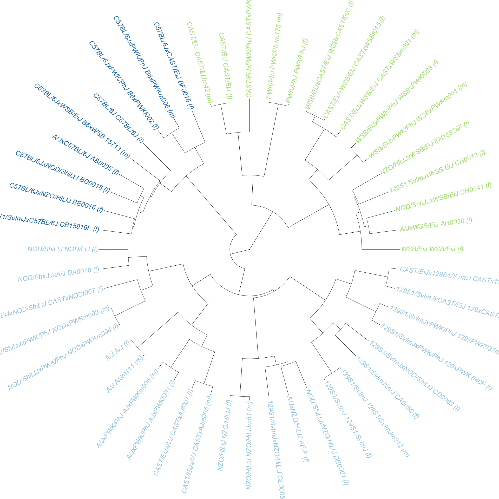
| Version | Author | Date |
|---|---|---|
| 3501596 | sam-widmayer | 2022-11-09 |
From here we curated a set of genotypes for each CC/DO founder strain that were fixed across replicate samples from that strain.
for(f in strict_founder_strains){

  print(paste("Generating Calls for",f))

  # Pulling the samples and genotypes for each CC/DO founder strain
  founder.geno.array <- final_founder_samples %>%
    dplyr::filter(dam == f,
                  sire == f) %>%
    # Attach all genotypes
    dplyr::left_join(.,genos.flagged, by = "sample") %>%
    # Use only high-quality markers
    dplyr::filter(marker_flag != "FLAG")


  # Count the number of unique allele calls for each marker
  founder.allele.counts <- founder.geno.array %>%
    dplyr::group_by(marker, genotype) %>%
    dplyr::count()

  # Collect markers which have identical genotypes across samples from the same founder
  complete_founder_genos <- founder.allele.counts %>%
    dplyr::filter(n == max(founder.allele.counts$n)) %>%
    dplyr::select(-n) %>%
    `colnames<-`(c("marker",f))

  # Assign these calls to a founder object
  assign(paste0("Calls_",f), complete_founder_genos)

}
[1] "Generating Calls for 129S1/SvImJ"
[1] "Generating Calls for A/J"
[1] "Generating Calls for C57BL/6J"
[1] "Generating Calls for CAST/EiJ"
[1] "Generating Calls for NOD/ShiLtJ"
[1] "Generating Calls for NZO/HILtJ"
[1] "Generating Calls for PWK/PhJ"
[1] "Generating Calls for WSB/EiJ"The genotypes for intersecting markers between two strains were combined (“crossed”) to form predicted genotypes for each F1 hybrid of CC/DO founders. Then, the genotypes of each CC/DO founder F1 hybrid were compared directly to what was predicted, and the concordance shown below is the proportion of markers of each individual that match this prediction.
# Build a list of founder consensus genotypes for good markers
founder_consensus_calls <- list(`Calls_A/J`, `Calls_C57BL/6J`, `Calls_129S1/SvImJ`, `Calls_NOD/ShiLtJ`,
                                `Calls_NZO/HILtJ`, `Calls_CAST/EiJ`, `Calls_PWK/PhJ`, `Calls_WSB/EiJ`)

# Generate a data frame with good markers as the sole column
good_markers <- genos.flagged %>%
  dplyr::distinct(marker, marker_flag) %>%
  dplyr::filter(marker_flag != "FLAG")

# Loop through the exisitng consensus calls and filter down to good markers
filtered_consensus_calls <- purrr::map(founder_consensus_calls,
                                       function(x){
                                         x %>%
                                           dplyr::filter(marker %in% good_markers$marker)
                                         }) %>%
  Reduce(full_join, .)

# Filter samples down to inbred strains and attach a proper strain name column
founder_sample_metadata <- final_founder_samples %>%
  dplyr::left_join(., sample.predicted.sexes.df) %>%
  dplyr::mutate(dam = as.character(dam),
                sire = as.character(sire),
                strain = if_else(dam == sire, true = dam, false = "CROSS"),
                resexed = if_else(predicted.sex != inferred.sex,
                                  true = "TRUE", false = "FALSE")) %>%
  dplyr::select(-inferred.sex)
#                 sample         dam        sire predicted.sex founder     bg      strain resexed
# 1:             A/J (f)         A/J         A/J             f FOUNDER INBRED         A/J   FALSE
# 2:         A/Jm111 (m)         A/J         A/J             m FOUNDER INBRED         A/J   FALSE
# 3:        C57BL/6J (f)    C57BL/6J    C57BL/6J             f FOUNDER INBRED    C57BL/6J    TRUE
# 4:     129S1/SvImJ (f) 129S1/SvImJ 129S1/SvImJ             f FOUNDER INBRED 129S1/SvImJ   FALSE
# 5: 129S1/SvImJm212 (m) 129S1/SvImJ 129S1/SvImJ             m FOUNDER INBRED 129S1/SvImJ   FALSE
# 6:         NOD/LtJ (f)  NOD/ShiLtJ  NOD/ShiLtJ             f FOUNDER INBRED  NOD/ShiLtJ   FALSE


# Create column index for intensity data tables
founder_samples_for_ints <- c("marker",founder_sample_metadata$sample)
founder_intensities <- founder_sample_metadata %>%
  dplyr::left_join(., long_intensities)
# First form a list of dams that comprise each F1 cross type
dams <- data.frame(tidyr::expand_grid(strict_founder_strains, strict_founder_strains, .name_repair = "minimal")) %>%
`colnames<-`(c("dams","sires")) %>%
# Select crosses between strains
# filter(dams != sires) %>%
dplyr::select(dams) %>%
as.list()
# Loop through the list of cross types and pull in genotype call objects
dam_calls <- list()
for(i in 1:length(dams$dams)){
dam_calls[[i]] <- get(ls(pattern = paste0("Calls_",dams$dams[i])))
}
# Do the same for the sires
sires <- data.frame(tidyr::expand_grid(strict_founder_strains, strict_founder_strains, .name_repair = "minimal")) %>%
`colnames<-`(c("dams","sires")) %>%
# filter(dams != sires) %>%
dplyr::select(sires) %>%
as.list()
sire_calls <- list()
for(i in 1:length(sires$sires)){
sire_calls[[i]] <- get(ls(pattern = paste0("Calls_",sires$sires[i])))
}
# Compare the predicted genotypes (from consensus calls) to the actual genotypes of each sample
# founder_background_QC(dam = dam_calls[[2]], sire = sire_calls[[2]])
bg_QC <- purrr::map2(dam_calls, sire_calls, founder_background_QC)[1] "Running QC: 129S1/SvImJ"
[1] "Running QC: (129S1/SvImJxA/J)F1"
[1] "Running QC: (129S1/SvImJxC57BL/6J)F1"
[1] "Running QC: (129S1/SvImJxCAST/EiJ)F1"
[1] "Running QC: (129S1/SvImJxNOD/ShiLtJ)F1"
[1] "Running QC: (129S1/SvImJxNZO/HILtJ)F1"
[1] "Running QC: (129S1/SvImJxPWK/PhJ)F1"
[1] "Running QC: (129S1/SvImJxWSB/EiJ)F1"
[1] "Running QC: (A/Jx129S1/SvImJ)F1"
[1] "Running QC: A/J"
[1] "Running QC: (A/JxC57BL/6J)F1"
[1] "Running QC: (A/JxCAST/EiJ)F1"
[1] "Running QC: (A/JxNOD/ShiLtJ)F1"
[1] "Running QC: (A/JxNZO/HILtJ)F1"
[1] "Running QC: (A/JxPWK/PhJ)F1"
[1] "Running QC: (A/JxWSB/EiJ)F1"
[1] "Running QC: (C57BL/6Jx129S1/SvImJ)F1"
[1] "Running QC: (C57BL/6JxA/J)F1"
[1] "Running QC: C57BL/6J"
[1] "Running QC: (C57BL/6JxCAST/EiJ)F1"
[1] "Running QC: (C57BL/6JxNOD/ShiLtJ)F1"
[1] "Running QC: (C57BL/6JxNZO/HILtJ)F1"
[1] "Running QC: (C57BL/6JxPWK/PhJ)F1"
[1] "Running QC: (C57BL/6JxWSB/EiJ)F1"
[1] "Running QC: (CAST/EiJx129S1/SvImJ)F1"
[1] "Running QC: (CAST/EiJxA/J)F1"
[1] "Running QC: (CAST/EiJxC57BL/6J)F1"
[1] "Running QC: CAST/EiJ"
[1] "Running QC: (CAST/EiJxNOD/ShiLtJ)F1"
[1] "Running QC: (CAST/EiJxNZO/HILtJ)F1"
[1] "Running QC: (CAST/EiJxPWK/PhJ)F1"
[1] "Running QC: (CAST/EiJxWSB/EiJ)F1"
[1] "Running QC: (NOD/ShiLtJx129S1/SvImJ)F1"
[1] "Running QC: (NOD/ShiLtJxA/J)F1"
[1] "Running QC: (NOD/ShiLtJxC57BL/6J)F1"
[1] "Running QC: (NOD/ShiLtJxCAST/EiJ)F1"
[1] "Running QC: NOD/ShiLtJ"
[1] "Running QC: (NOD/ShiLtJxNZO/HILtJ)F1"
[1] "Running QC: (NOD/ShiLtJxPWK/PhJ)F1"
[1] "Running QC: (NOD/ShiLtJxWSB/EiJ)F1"
[1] "Running QC: (NZO/HILtJx129S1/SvImJ)F1"
[1] "Running QC: (NZO/HILtJxA/J)F1"
[1] "Running QC: (NZO/HILtJxC57BL/6J)F1"
[1] "Running QC: (NZO/HILtJxCAST/EiJ)F1"
[1] "Running QC: (NZO/HILtJxNOD/ShiLtJ)F1"
[1] "Running QC: NZO/HILtJ"
[1] "Running QC: (NZO/HILtJxPWK/PhJ)F1"
[1] "Running QC: (NZO/HILtJxWSB/EiJ)F1"
[1] "Running QC: (PWK/PhJx129S1/SvImJ)F1"
[1] "Running QC: (PWK/PhJxA/J)F1"
[1] "Running QC: (PWK/PhJxC57BL/6J)F1"
[1] "Running QC: (PWK/PhJxCAST/EiJ)F1"
[1] "Running QC: (PWK/PhJxNOD/ShiLtJ)F1"
[1] "Running QC: (PWK/PhJxNZO/HILtJ)F1"
[1] "Running QC: PWK/PhJ"
[1] "Running QC: (PWK/PhJxWSB/EiJ)F1"
[1] "Running QC: (WSB/EiJx129S1/SvImJ)F1"
[1] "Running QC: (WSB/EiJxA/J)F1"
[1] "Running QC: (WSB/EiJxC57BL/6J)F1"
[1] "Running QC: (WSB/EiJxCAST/EiJ)F1"
[1] "Running QC: (WSB/EiJxNOD/ShiLtJ)F1"
[1] "Running QC: (WSB/EiJxNZO/HILtJ)F1"
[1] "Running QC: (WSB/EiJxPWK/PhJ)F1"
[1] "Running QC: WSB/EiJ"# Keep outputs from the QC that are lists; if QC wasn't performed for a given background, the output was a character vector warning
founder_background_QC_tr <- bg_QC %>%
purrr::keep(., is.list) %>%
# Instead of having 64 elements of lists of two, have two lists of 64:
# 1) All good genotypes from each cross with concordance values
# 2) All concordance summaries for each cross
purrr::transpose(.)
# Bind together all concordance summaries
founder_concordance_df <- Reduce(rbind, founder_background_QC_tr[[2]])
# If all markers for a given chromosome type were either concordant or discordant, NAs are returned
# This step assigns those NA values a 0
founder_concordance_df[is.na(founder_concordance_df)] <- 0
# Form concordance as a percentage
founder_concordance_df_2 <- founder_concordance_df %>%
dplyr::mutate(concordance = MATCH/(MATCH + `NO MATCH`)) %>%
dplyr::mutate(dam = gsub(dam, pattern = "[.]", replacement = "/"),
sire = gsub(sire, pattern = "[.]", replacement = "/"))
founder_concordance_df_2$alt_chr <- factor(founder_concordance_df_2$alt_chr,
levels = c("Autosome","X","Y","M","Other"))
founder_concordance_df_3 <- founder_concordance_df_2 %>%
dplyr::filter(alt_chr == "Autosome")
founder_palette <- qtl2::CCcolors
names(founder_palette) <- strict_founder_strains[c(2,3,1,5,6,4,7,8)]
founder_palette_2 <- founder_palette
# Plot Autosomal Concordance
concordance_plot <- ggplot(founder_concordance_df_3, mapping = aes(x = dam, y = concordance, color = dam, fill = sire)) +
geom_jitter(shape = 21, width = 0.25) +
scale_fill_manual(values = founder_palette_2) +
scale_colour_manual(values = founder_palette_2) +
ylim(c(0.5,1.05)) +
labs(x = "Dam Founder Strain",
y = "Autosomal Genotype Concordance") +
QCtheme
ggplotly(concordance_plot)# Plot X Chromosome Concordance
concordance_plot <- ggplot(founder_concordance_df_2 %>%
dplyr::filter(alt_chr == "X"),
mapping = aes(x = dam, y = concordance, color = dam, fill = sire)) +
geom_jitter(shape = 21, width = 0.25) +
scale_fill_manual(values = founder_palette_2) +
scale_colour_manual(values = founder_palette_2) +
ylim(c(0.5,1.05)) +
labs(x = "Dam Founder Strain",
y = "X Chromosome Genotype Concordance") +
QCtheme
ggplotly(concordance_plot)Writing reference files
The list of output file types following QC is as follows:
Genotype file; rows = markers, columns = samples
Probe intensity file; rows = markers, columns = samples
Sample metadata; columns = sample, strain, sex
Each file type is generated for:
All good samples
Eight CC/DO founder strains
In total, 7762 markers and 53 samples passed the QC steps we imposed, and wrote these genotype data and metadata to new reference files.
# Writing output files
dir.create("output", showWarnings = F)
dir.create("output/MUGA", showWarnings = F)

write.csv(reference_genos_all_samples,
  file = "output/MUGA/MUGA_genotypes.csv",
  row.names = F)
system("gzip output/MUGA/MUGA_genotypes.csv")

write.csv(reference_xints_all_samples,
  file = "output/MUGA/MUGA_x_intensities.csv",
  row.names = F)
system("gzip output/MUGA/MUGA_x_intensities.csv")

write.csv(reference_yints_all_samples,
  file = "output/MUGA/MUGA_y_intensities.csv",
  row.names = F)
system("gzip output/MUGA/MUGA_y_intensities.csv")

write.csv(strain_assignment,
  file = "output/MUGA/MUGA_sample_metadata.csv",
  row.names = F)

write.csv(final_founder_consensus_genotypes,
  file = "output/MUGA/MUGA_founder_consensus_genotypes.csv",
  row.names = F)
system("gzip output/MUGA/MUGA_founder_consensus_genotypes.csv")

write.csv(founder_xints,
  file = "output/MUGA/MUGA_founder_mean_x_intensities.csv",
  row.names = F)
system("gzip output/MUGA/MUGA_founder_mean_x_intensities.csv")

write.csv(founder_yints,
  file = "output/MUGA/MUGA_founder_mean_y_intensities.csv",
  row.names = F)
system("gzip output/MUGA/MUGA_founder_mean_y_intensities.csv")

write.csv(founder_sample_metadata_conc,
            file = "output/MUGA/MUGA_founder_metadata.csv",
            row.names = F)
sessionInfo()R version 4.2.1 (2022-06-23)
Platform: x86_64-apple-darwin17.0 (64-bit)
Running under: macOS Big Sur ... 10.16
Matrix products: default
BLAS: /Library/Frameworks/R.framework/Versions/4.2/Resources/lib/libRblas.0.dylib
LAPACK: /Library/Frameworks/R.framework/Versions/4.2/Resources/lib/libRlapack.dylib
locale:
[1] en_US.UTF-8/en_US.UTF-8/en_US.UTF-8/C/en_US.UTF-8/en_US.UTF-8
attached base packages:
[1] stats graphics grDevices utils datasets methods base
other attached packages:
[1] vroom_1.6.0 tictoc_1.1 RColorBrewer_1.1-3 ape_5.6-2
[5] progress_1.2.2 plotly_4.10.1 ggplot2_3.4.0 DT_0.26
[9] magrittr_2.0.3 qtl2_0.28 furrr_0.3.1 future_1.29.0
[13] purrr_0.3.5 data.table_1.14.4 stringr_1.4.1 tidyr_1.2.1
[17] dplyr_1.0.10
loaded via a namespace (and not attached):
[1] httr_1.4.4 sass_0.4.2 bit64_4.0.5 jsonlite_1.8.3
[5] viridisLite_0.4.1 bslib_0.4.1 assertthat_0.2.1 highr_0.9
[9] blob_1.2.3 yaml_2.3.6 globals_0.16.1 pillar_1.8.1
[13] RSQLite_2.2.18 lattice_0.20-45 glue_1.6.2 digest_0.6.30
[17] promises_1.2.0.1 colorspace_2.0-3 htmltools_0.5.3 httpuv_1.6.6
[21] pkgconfig_2.0.3 listenv_0.8.0 scales_1.2.1 whisker_0.4
[25] later_1.3.0 tzdb_0.3.0 git2r_0.30.1 tibble_3.1.8
[29] farver_2.1.1 generics_0.1.3 ellipsis_0.3.2 cachem_1.0.6
[33] withr_2.5.0 lazyeval_0.2.2 cli_3.4.1 crayon_1.5.2
[37] memoise_2.0.1 evaluate_0.18 fs_1.5.2 fansi_1.0.3
[41] parallelly_1.32.1 nlme_3.1-157 tools_4.2.1 prettyunits_1.1.1
[45] hms_1.1.2 lifecycle_1.0.3 munsell_0.5.0 compiler_4.2.1
[49] jquerylib_0.1.4 rlang_1.0.6 grid_4.2.1 rstudioapi_0.14
[53] htmlwidgets_1.5.4 crosstalk_1.2.0 labeling_0.4.2 rmarkdown_2.18
[57] gtable_0.3.1 codetools_0.2-18 DBI_1.1.3 R6_2.5.1
[61] knitr_1.40 fastmap_1.1.0 bit_4.0.4 utf8_1.2.2
[65] workflowr_1.7.0 rprojroot_2.0.3 stringi_1.7.8 parallel_4.2.1
[69] Rcpp_1.0.9 vctrs_0.5.0 tidyselect_1.2.0 xfun_0.34