Reference Data QC: MegaMUGA
Last updated: 2023-01-13
Checks: 6 1
Knit directory: MUGA_reference_data/
This reproducible R Markdown analysis was created with workflowr (version 1.7.0). The Checks tab describes the reproducibility checks that were applied when the results were created. The Past versions tab lists the development history.
The R Markdown file has unstaged changes. To know which version of
the R Markdown file created these results, you’ll want to first commit
it to the Git repo. If you’re still working on the analysis, you can
ignore this warning. When you’re finished, you can run
wflow_publish to commit the R Markdown file and build the
HTML.
Great job! The global environment was empty. Objects defined in the global environment can affect the analysis in your R Markdown file in unknown ways. For reproduciblity it’s best to always run the code in an empty environment.
The command set.seed(20221108) was run prior to running
the code in the R Markdown file. Setting a seed ensures that any results
that rely on randomness, e.g. subsampling or permutations, are
reproducible.
Great job! Recording the operating system, R version, and package versions is critical for reproducibility.
Nice! There were no cached chunks for this analysis, so you can be confident that you successfully produced the results during this run.
Great job! Using relative paths to the files within your workflowr project makes it easier to run your code on other machines.
Great! You are using Git for version control. Tracking code development and connecting the code version to the results is critical for reproducibility.
The results in this page were generated with repository version 83baed5. See the Past versions tab to see a history of the changes made to the R Markdown and HTML files.
Note that you need to be careful to ensure that all relevant files for
the analysis have been committed to Git prior to generating the results
(you can use wflow_publish or
wflow_git_commit). workflowr only checks the R Markdown
file, but you know if there are other scripts or data files that it
depends on. Below is the status of the Git repository when the results
were generated:
Ignored files:
    Ignored:    .DS_Store
    Ignored:    .Rhistory
    Ignored:    .Rproj.user/
    Ignored:    code/.DS_Store
    Ignored:    data/.DS_Store
    Ignored:    output/.DS_Store
    Ignored:    output/MUGA/.DS_Store
    Ignored:    output/MegaMUGA/.DS_Store

Untracked files:
    Untracked:  README.html
    Untracked:  code/README.html
    Untracked:  data/GigaMUGA/FPGM_1-6_FinalReport.txt
    Untracked:  data/GigaMUGA/FPGM_1-6_FinalReport.zip
    Untracked:  data/GigaMUGA/GC_15_F_ReSex_Results/
    Untracked:  data/GigaMUGA/GigaMUGA_control_genotypes.txt
    Untracked:  data/GigaMUGA/GigaMUGA_founder_consensus_genotypes/
    Untracked:  data/GigaMUGA/GigaMUGA_founder_sample_concordance/
    Untracked:  data/GigaMUGA/GigaMUGA_founder_sample_dendrogram_genos/
    Untracked:  data/GigaMUGA/GigaMUGA_founder_sample_genotypes/
    Untracked:  data/GigaMUGA/GigaMUGA_reference_genotypes/
    Untracked:  output/GigaMUGA/
    Untracked:  output/MUGA/MUGA_founder_consensus_genotypes.csv
    Untracked:  output/MUGA/MUGA_founder_mean_x_intensities.csv
    Untracked:  output/MUGA/MUGA_founder_mean_y_intensities.csv
    Untracked:  output/MUGA/MUGA_genotypes.csv
    Untracked:  output/MUGA/MUGA_x_intensities.csv
    Untracked:  output/MUGA/MUGA_y_intensities.csv

Unstaged changes:
    Modified:   analysis/MegaMUGA_Reference_QC.Rmd
    Deleted:    code/workflowr_build.R
    Modified:   output/MUGA/MUGA_founder_consensus_genotypes.csv.gz
    Modified:   output/MUGA/MUGA_founder_mean_x_intensities.csv.gz
    Modified:   output/MUGA/MUGA_founder_mean_y_intensities.csv.gz
    Modified:   output/MUGA/MUGA_founder_metadata.csv
    Modified:   output/MUGA/MUGA_genotypes.csv.gz
    Modified:   output/MUGA/MUGA_sample_metadata.csv
    Modified:   output/MUGA/MUGA_x_intensities.csv.gz
    Modified:   output/MUGA/MUGA_y_intensities.csv.gz
    Deleted:    output/MegaMUGA/MegaMUGA_founder_consensus_genotypes.csv.gz
    Deleted:    output/MegaMUGA/MegaMUGA_founder_mean_x_intensities.csv.gz
    Deleted:    output/MegaMUGA/MegaMUGA_founder_mean_y_intensities.csv.gz
    Deleted:    output/MegaMUGA/MegaMUGA_founder_metadata.csv
    Deleted:    output/MegaMUGA/MegaMUGA_genotypes.csv.gz
    Deleted:    output/MegaMUGA/MegaMUGA_sample_metadata.csv
    Deleted:    output/MegaMUGA/MegaMUGA_x_intensities.csv.gz
    Deleted:    output/MegaMUGA/MegaMUGA_y_intensities.csv.gz
Note that any generated files, e.g. HTML, png, CSS, etc., are not included in this status report because it is ok for generated content to have uncommitted changes.
These are the previous versions of the repository in which changes were
made to the R Markdown (analysis/MegaMUGA_Reference_QC.Rmd)
and HTML (docs/MegaMUGA_Reference_QC.html) files. If you’ve
configured a remote Git repository (see ?wflow_git_remote),
click on the hyperlinks in the table below to view the files as they
were in that past version.
| File | Version | Author | Date | Message |
|---|---|---|---|---|
| Rmd | 83baed5 | sam-widmayer | 2023-01-13 | overwrite csvs |
| Rmd | 877e958 | sam-widmayer | 2023-01-13 | ref data changes for GEDI link |
| html | 025f6f8 | sam-widmayer | 2022-11-09 | Build site. |
| Rmd | d352284 | sam-widmayer | 2022-11-09 | update site theme and fold code snippets |
| html | d352284 | sam-widmayer | 2022-11-09 | update site theme and fold code snippets |
| Rmd | 3501596 | sam-widmayer | 2022-11-09 | change site theme and add index tables |
| html | 3501596 | sam-widmayer | 2022-11-09 | change site theme and add index tables |
| Rmd | 1074529 | sam-widmayer | 2022-11-08 | update markdown formatting for workflowr |
| Rmd | efe8849 | sam-widmayer | 2022-11-08 | initialize workflowr integration |
MegaMUGA Annotations
Reading in reference genotypes and metadata
First I read in the reference sample genotypes, as well as marker annotations from an analysis previously conducted by Karl Broman, Dan Gatti, and Belinda Cornes.
# Reading in reference sample genotype data
control_genotypes <- suppressWarnings(data.table::fread(cmd = "unzip -cq data/MegaMUGA/control.genotypes.csv.zip",
                                                        check.names = T))
colnames(control_genotypes)[1] <- "marker"

# Later in analysis, lowercase "i" in strain ID eliminates a founder sample from background QC
colnames(control_genotypes)[which(str_detect(colnames(control_genotypes), pattern = "NZO.HiLtJm36511"))] <- "NZO.HILtJm36511"

## Reading in marker annotations fro Broman, Gatti, & Cornes analysis
mm_metadata <- data.table::fread("data/MegaMUGA/mm_uwisc_v2.csv")
Marker QC: Searching for missing genotype calls
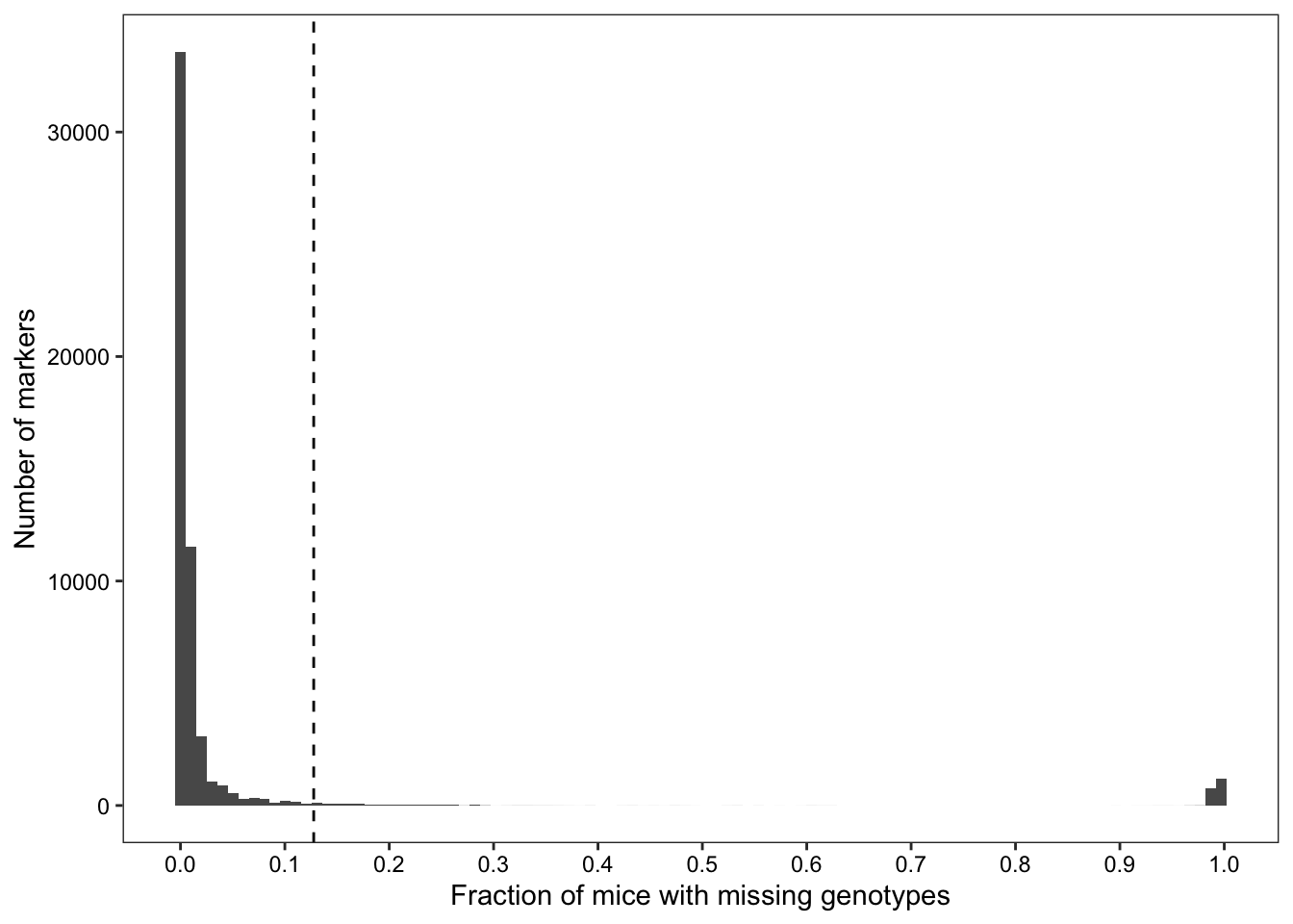
We searched for probes where many mice are missing genotype calls.
## Calculating allele frequencies for each marker
control_allele_freqs <- control_genotypes %>%
  tidyr::pivot_longer(-marker, names_to = "sample", values_to = "genotype") %>%
  dplyr::group_by(marker, genotype) %>%
  dplyr::count() %>%
  # Result: number of genotype calls for each marker across all samples
  # i.e.
  #  marker            genotype     n
  #  B6_01-033811444-S A            8
  #  B6_01-033811444-S H            2
  #  B6_01-033811444-S N            1

  dplyr::ungroup() %>%
  dplyr::group_by(marker) %>%
  dplyr::mutate(freq = round(n/sum(n), 3),
                genotype = as.factor(genotype)) %>%
  # Result: allele frequency calls for each marker across all samples
  # i.e.
#  marker            genotype   n  freq
#  B6_01-033811444-S        A   8 0.022
#  B6_01-033811444-S        H   2 0.005
#  B6_01-033811444-S        N   1 0.003
#  B6_01-033811444-S        T 353 0.970
  dplyr::left_join(., mm_metadata)


## Filtering to markers with missing genotypes
no.calls <- control_allele_freqs %>%
  dplyr::ungroup() %>%
  dplyr::filter(genotype == "N") %>%
  tidyr::pivot_wider(names_from = genotype,
                     values_from = n) %>%
  dplyr::select(marker, chr, bp_grcm39, freq) %>%
  dplyr::mutate(chr = as.factor(chr))


## Identifying markers with missing genotypes at a frequency higher than the 95th percentile of "N" frequencies across all markers
cutoff <- quantile(no.calls$freq, probs = seq(0,1,0.05))[[20]]
above.cutoff <- no.calls %>%
  dplyr::filter(freq > cutoff)
Of 77808 markers, 54990 failed to genotype at least one sample, and 2750 markers failed to genotype at least 12.765% of samples.
| Version | Author | Date |
|---|---|---|
| 3501596 | sam-widmayer | 2022-11-09 |
Sample QC
Searching for samples with poor marker representation
In a similar fashion, we calculated the number of reference samples with missing genotypes. Repeated observations of samples/strains with identical names meant that genotype counts for each marker among them couldn’t be grouped and tallied, so determining no-call frequency occurred column-wise. Mouse over individual samples to see the number of markers with missing genotypes for each sample.
## Calculating the number of missing markers for each sample
n.calls.strains <- apply(X = control_genotypes[,2:ncol(control_genotypes)],
                         MARGIN = 2,
                         function(x) table(x)[5])
n.calls.strains.df <- data.frame(n.calls.strains)
n.calls.strains.df$sample <- names(n.calls.strains)
n.calls.strains.df %<>%
  dplyr::rename(n.no.calls = n.calls.strains)
# n.no.calls                                   sample
# 2355                       (129S1/SvImJxA/J)F1f0056
# 2204                       (129S1/SvImJxA/J)F1f0056
# 2171                 (129S1/SvImJxC57BL/6J)F1f15916
# 2348                 (129S1/SvImJxC57BL/6J)F1m15914
# 2232                   (129S1/SvImJxCAST/EiJ)F1f005
# 2328                   (129S1/SvImJxCAST/EiJ)F1m002
# 2291                (129S1/SvImJxNOD/ShiLtJ)F1f0063
# 2197                 (129S1/SvImJxNZO/HILtJ)F1f0005
# 2316                 (129S1/SvImJxNZO/HILtJ)F1m0004


## Interactive plot of the number of missing genotypes for each sample.
bad_sample_cutoff <- quantile(n.calls.strains.df$n.no.calls, probs = seq(0,1,0.05))[20]
high.n.samples <- n.calls.strains.df %>%
  dplyr::filter(n.no.calls > bad_sample_cutoff)
sampleQC <- ggplot(n.calls.strains.df,
                   mapping = aes(x = reorder(sample,n.no.calls),
                                 y = n.no.calls,
                                 text = paste("Sample:", sample))) +
  geom_point() +
  QCtheme +
  theme(axis.text.x = element_blank(),
        axis.ticks.x = element_blank()) +
  geom_hline(yintercept = bad_sample_cutoff, linetype = 2) +
  labs(x = "Number of mice with missing genotypes",
       y = "Number of markers")
ggplotly(sampleQC, tooltip = c("text","y"))
Validating sex of reference samples
We next validated the sexes of each sample using sex chromosome probe intensities. We paired up probe intensities, joined available metadata, and filtered down to only markers covering the X and Y chromosomes.
## Reading in genotype intensities
x_intensities <- suppressWarnings(data.table::fread(cmd = "unzip -cq data/MegaMUGA/control.X.csv.zip",
                                                        check.names = T))
colnames(x_intensities)[1] <- "marker"
colnames(x_intensities)[which(str_detect(colnames(x_intensities), pattern = "NZO.HiLtJm36511"))] <- "NZO.HILtJm36511"

y_intensities <- suppressWarnings(data.table::fread(cmd = "unzip -cq data/MegaMUGA/control.Y.csv.zip",
                                                        check.names = T))
colnames(y_intensities)[1] <- "marker"
colnames(y_intensities)[which(str_detect(colnames(y_intensities), pattern = "NZO.HiLtJm36511"))] <- "NZO.HILtJm36511"

## Check to see if dimensions of intensity tables are identical, marker orders identical, and sample orders identical
if((unique(dim(x_intensities) == dim(y_intensities)) &&
   unique(colnames(x_intensities) == colnames(y_intensities)) &&
   unique(x_intensities$marker == y_intensities$marker)) == TRUE){
     ## Pivoting the data longer
  x_int_long <- x_intensities %>%
  tidyr::pivot_longer(cols = -marker,
                      names_to = "sample",
                      values_to = "x_int")
  y_int_long <- y_intensities %>%
  tidyr::pivot_longer(cols = -marker,
                      names_to = "sample",
                      values_to = "y_int")

  long_intensities <- cbind(x_int_long, y_int_long)
} else {
     print("Source intensity data frames have non-identical structure; exiting")
}

## Joining slimmer intensity files with marker metadata and reducing to markers on sex chromosomes
long_XY_intensities <- long_intensities[,c(1,2,3,6)] %>%
  dplyr::left_join(., mm_metadata) %>%
  dplyr::filter(chr %in% c("X","Y"))

# Expected output
# marker                          ample x_int y_int chr   bp_mm10 bp_grcm39   cM_cox strand snp unique
# XiD1       X.129S1.SvImJxA.J.F1f0056 1.161 0.094   X 102827921 101871527 44.17434   plus  TG   TRUE
# XiD1     X.129S1.SvImJxA.J.F1f0056.1 1.034 0.054   X 102827921 101871527 44.17434   plus  TG   TRUE
# XiD1 X.129S1.SvImJxC57BL.6J.F1f15916 0.805 0.068   X 102827921 101871527 44.17434   plus  TG   TRUE
# XiD1 X.129S1.SvImJxC57BL.6J.F1m15914 0.371 0.035   X 102827921 101871527 44.17434   plus  TG   TRUE
# XiD1   X.129S1.SvImJxCAST.EiJ.F1f005 0.696 0.040   X 102827921 101871527 44.17434   plus  TG   TRUE
# XiD1   X.129S1.SvImJxCAST.EiJ.F1m002 0.591 0.041   X 102827921 101871527 44.17434   plus  TG   TRUE
# unmapped                                            probe strand_flipped
# FALSE CTGCCTTCAAAAGTGCTGGGATTAAAATGATGAGCGAGCAATGCCCAGCC          FALSE
# FALSE CTGCCTTCAAAAGTGCTGGGATTAAAATGATGAGCGAGCAATGCCCAGCC          FALSE
# FALSE CTGCCTTCAAAAGTGCTGGGATTAAAATGATGAGCGAGCAATGCCCAGCC          FALSE
# FALSE CTGCCTTCAAAAGTGCTGGGATTAAAATGATGAGCGAGCAATGCCCAGCC          FALSE
# FALSE CTGCCTTCAAAAGTGCTGGGATTAAAATGATGAGCGAGCAATGCCCAGCC          FALSE
# FALSE CTGCCTTCAAAAGTGCTGGGATTAAAATGATGAGCGAGCAATGCCCAGCC          FALSE
Then we flagged markers with high missingness across all samples, as well as samples with high missingness among all markers.
## Flagging markers and samples based on previous QC steps
flagged_XY_intensities <- long_XY_intensities %>%
  dplyr::mutate(marker_flag = dplyr::if_else(condition = marker %in% above.cutoff$marker,
                                             true = "FLAG",
                                             false = "")) %>%
  dplyr::mutate(high_missing_sample = dplyr::if_else(condition = sample %in% high.n.samples$sample,
                                                     true = "FLAG",
                                                     false = ""))
The first round of inferring predicted sexes used a rough search of the sample name for expected nomenclature convention, which includes a sex denotation.
## First round of predicted sex inference
## Input: flagged XY intensities
prelim.predicted.sexes <- flagged_XY_intensities %>%
dplyr::mutate(bg = dplyr::case_when(stringr::str_detect(string = sample,
pattern = "F1") == TRUE ~ "F1",
TRUE ~ "unknown"),
predicted.sex = dplyr::case_when(stringr::str_detect(string = sample,
pattern = "F1f") == TRUE ~ "f",
stringr::str_detect(string = sample,
pattern = "F1m") == TRUE ~ "m",
TRUE ~ "unknown"))
## Output: flagged intensities with preliminary sex predictions and background assignments among F1 hybrids
# prelim.predicted.sexes[764:789,] %>%
# dplyr::select(marker, sample, marker_flag, high_missing_sample, predicted.sex)
# marker sample marker_flag high_missing_sample predicted.sex
# 764 XiE2 X.C57BL.6JxNOD.ShiLtJ.F1f0018 FLAG f
# 765 XiE2 X.C57BL.6JxNZO.HILtJ.F1f0016 FLAG f
# 766 XiE2 X.C57BL.6JxNZO.HILtJ.F1m15853 FLAG m
# 767 XiE2 X.C57BL.6JxPWK.PhJ.F1f002 FLAG f
# 768 XiE2 X.C57BL.6JxPWK.PhJ.F1m005 FLAG m
# 769 XiE2 X.C57BL.6JxPWK.PhJ.F1m005.1 FLAG m
# 770 XiE2 X.C57BL.6JxSJL.J.F1m35973 FLAG FLAG m
# 771 XiE2 X.C57BL.6JxWSB.EiJ.F1f0300 FLAG f
# 772 XiE2 X.C57BL.6JxWSB.EiJ.F1m15714 FLAG m
# 773 XiE2 X.CAST.EiJx129S1.SvImJ.F1f012 FLAG f
# 774 XiE2 X.CAST.EiJx129S1.SvImJ.F1m001 FLAG m
# 775 XiE2 X.CAST.EiJxA.J.F1f002 FLAG f
# 776 XiE2 X.CAST.EiJxA.J.F1f002.1 FLAG f
# 777 XiE2 X.CAST.EiJxA.J.F1m005 FLAG m
# 778 XiE2 X.CAST.EiJxC57BL.6J.F1m FLAG m
# 779 XiE2 X.CAST.EiJxC57BL.6J.F1m.1 FLAG m
# 780 XiE2 X.CAST.EiJxNOD.ShiLtJ.F1f007 FLAG f
# 781 XiE2 X.CAST.EiJxNOD.ShiLtJ.F1f007.1 FLAG f
# 782 XiE2 X.CAST.EiJxNZO.HILtJ.F1f FLAG f
# 783 XiE2 X.CAST.EiJxNZO.HILtJ.F1f.1 FLAG f
# 784 XiE2 X.CAST.EiJxNZO.HILtJ.F1m FLAG m
# 785 XiE2 X.CAST.EiJxNZO.HILtJ.F1m.1 FLAG m
# 786 XiE2 X.CAST.EiJxPWK.PhJ.F10123 FLAG unknown
# 787 XiE2 X.CAST.EiJxPWK.PhJ.F1f0163 FLAG f
# 788 XiE2 X.CAST.EiJxWSB.EiJ.F1f0113 FLAG f
# 789 XiE2 X.CAST.EiJxWSB.EiJ.F1m0096 FLAG m
## Filtering down to samples without preliminary sex predictions
unknown <- prelim.predicted.sexes %>%
dplyr::filter(predicted.sex == "unknown")
## Using regex searching of sample IDs to deduce the sex of each sample
###########################################################
## Key processes and expected outputs at each iteration: ##
###########################################################
#####################################################################
## 1) Extracting the a substring of X digits into the sample name. ##
#####################################################################
# mouse.id.X = stringr::str_sub(sample, -X)
# i.e.)
# unknown %>%
# dplyr::mutate(mouse.id.3 = stringr::str_sub(sample, -3)) %>%
# dplyr::select(sample, mouse.id.3) %>%
# head(10)
# sample mouse.id.3
# 1 X.CAST.EiJxPWK.PhJ.F10123 123
# 2 X017.FH.F1 .F1
# 3 X124S4.SvJaeJm39510 510
# 4 X129P1.ReJm35858 858
# 5 X129P2.OlaHsdm sdm
# 6 X129P2.OlaHsdm.1 m.1
# 7 X129P3.Jm37959 959
# 8 X129S1.SvImJf mJf
# 9 X129S1.SvImJf.1 f.1
# 10 X129S1.SvImJf0827 827
#####################################################################################
## 2) Assigning the predicted sex based on expected mouse nomenclature convention. ##
#####################################################################################
# predicted.sex.X = dplyr::case_when(stringr::str_sub(mouse.id.X, 1, 1) %in% c("m","M") ~ "m", stringr::str_sub(mouse.id.X, 1, 1) %in% c("f","F") ~ "f", TRUE ~ "unknown")
# i.e.)
# unknown %>%
# dplyr::mutate(mouse.id.5= stringr::str_sub(sample, -5),
# predicted.sex.5 =
# dplyr::case_when(stringr::str_sub(mouse.id.5, 1, 1) %in% c("m","M") ~ "m",
# stringr::str_sub(mouse.id.5, 1, 1) %in% c("f","F") ~ "f",
# ` TRUE ~ "unknown")) %>%
# dplyr::select(sample, mouse.id.5, predicted.sex.5) %>% head(14)
# sample mouse.id.5 predicted.sex.5
# 1 X.CAST.EiJxPWK.PhJ.F10123 10123 unknown
# 2 X017.FH.F1 FH.F1 f
# 3 X124S4.SvJaeJm39510 39510 unknown
# 4 X129P1.ReJm35858 35858 unknown
# 5 X129P2.OlaHsdm aHsdm unknown
# 6 X129P2.OlaHsdm.1 sdm.1 unknown
# 7 X129P3.Jm37959 37959 unknown
# 8 X129S1.SvImJf vImJf unknown
# 9 X129S1.SvImJf.1 mJf.1 m
# 10 X129S1.SvImJf0827 f0827 f
# 11 X129S1.SvImJf0827.1 827.1 unknown
# 12 X129S1.SvImJm vImJm unknown
# 13 X129S1.SvImJm.1 mJm.1 m
# 14 X129S1.SvImJm1314 m1314 m
##############################################################################################
# 3) Inferring the strain background by removing the mouse id from the sample name when a sex is predicted. In certain cases, symbols had to be extracted prior to sex and background inference.
##############################################################################################
# bg = if_else(condition = (predicted.sex.X == "m" | predicted.sex.X == "f"),
# true = str_replace(string = bg,
# pattern = mouse.id.X,
# replacement = ""),
# false = bg)
# i.e.)
# unknown %>%
# dplyr::mutate(mouse.id.5 = stringr::str_sub(sample, -5),
# mouse.id.5 = stringr::str_replace(string = mouse.id.5,
# pattern = "[:symbol:]",
# replacement = ""),
# predicted.sex.5 = dplyr::case_when(stringr::str_sub(mouse.id.5, 1, 1) %in% c("m","M") ~ "m",
# stringr::str_sub(mouse.id.5, 1, 1) %in% c("f","F") ~ "f",
# TRUE ~ "unknown"),
# bg = if_else(condition = (predicted.sex.5 == "m" | predicted.sex.5 == "f"),
# true = str_replace(string = bg,
# pattern = mouse.id.5,
# replacement = ""),
# false = bg)) %>%
# dplyr::select(sample, mouse.id.5, predicted.sex.5, bg) %>% head(14)
# sample mouse.id.5 predicted.sex.5 bg
# 1 X.CAST.EiJxPWK.PhJ.F10123 10123 unknown F1
# 2 X017.FH.F1 FH.F1 f F1
# 3 X124S4.SvJaeJm39510 39510 unknown X124S4.SvJaeJm39510
# 4 X129P1.ReJm35858 35858 unknown X129P1.ReJm35858
# 5 X129P2.OlaHsdm aHsdm unknown X129P2.OlaHsdm
# 6 X129P2.OlaHsdm.1 sdm.1 unknown X129P2.OlaHsdm.1
# 7 X129P3.Jm37959 37959 unknown X129P3.Jm37959
# 8 X129S1.SvImJf vImJf unknown X129S1.SvImJf
# 9 X129S1.SvImJf.1 mJf.1 m X129S1.SvI
# 10 X129S1.SvImJf0827 f0827 f X129S1.SvImJ
# 11 X129S1.SvImJf0827.1 827.1 unknown X129S1.SvImJf0827.1
# 12 X129S1.SvImJm vImJm unknown X129S1.SvImJm
# 13 X129S1.SvImJm.1 mJm.1 m X129S1.SvI
# 14 X129S1.SvImJm1314 m1314 m X129S1.SvImJ
digit.trim <- unknown %>%
# One character
dplyr::mutate(mouse.id.1 = stringr::str_sub(sample, -1),
predicted.sex.1 = dplyr::case_when(stringr::str_sub(mouse.id.1, 1, 1) %in% c("m","M") ~ "m",
stringr::str_sub(mouse.id.1, 1, 1) %in% c("f","F") ~ "f",
TRUE ~ "unknown"),
# Three characters
mouse.id.3= stringr::str_sub(sample, -3),
predicted.sex.3 = dplyr::case_when(stringr::str_sub(mouse.id.3, 1, 1) %in% c("m","M") ~ "m",
stringr::str_sub(mouse.id.3, 1, 1) %in% c("f","F") ~ "f",
TRUE ~ "unknown"),
# Four characters
mouse.id.4 = stringr::str_sub(sample, -4),
predicted.sex.4 = dplyr::case_when(stringr::str_sub(mouse.id.4, 1, 1) %in% c("m","M") ~ "m",
stringr::str_sub(mouse.id.4, 1, 1) %in% c("f","F") ~ "f",
TRUE ~ "unknown"),
# Five characters
mouse.id.5 = stringr::str_sub(sample, -5),
mouse.id.5 = stringr::str_replace(string = mouse.id.5, ## a couple symbols in these ids mess up the regex search
pattern = "[:symbol:]",
replacement = ""),
predicted.sex.5 = dplyr::case_when(stringr::str_sub(mouse.id.5, 1, 1) %in% c("m","M") ~ "m",
stringr::str_sub(mouse.id.5, 1, 1) %in% c("f","F") ~ "f",
TRUE ~ "unknown"),
# Six characters
mouse.id.6 = stringr::str_sub(sample, -6),
mouse.id.6 = stringr::str_replace(string = mouse.id.6, ## a couple symbols in these ids mess up the regex search
pattern = "[:punct:]",
replacement = ""),
mouse.id.6 = stringr::str_replace(string = mouse.id.6, ## a couple symbols in these ids mess up the regex search
pattern = "[:symbol:]",
replacement = ""),
predicted.sex.6 = dplyr::case_when(stringr::str_sub(mouse.id.6, 1, 1) %in% c("m","M") ~ "m",
stringr::str_sub(mouse.id.6, 1, 1) %in% c("f","F") ~ "f",
TRUE ~ "unknown"),
# Seven characters
mouse.id.7 = stringr::str_sub(sample, -7),
mouse.id.7 = stringr::str_replace(string = mouse.id.7, ## a couple symbols in these ids mess up the regex search
pattern = "[:punct:]",
replacement = ""),
mouse.id.7 = stringr::str_replace(string = mouse.id.7, ## a couple symbols in these ids mess up the regex search
pattern = "[:symbol:]",
replacement = ""),
predicted.sex.7 = dplyr::case_when(stringr::str_sub(mouse.id.7, 1, 1) %in% c("m","M") ~ "m",
stringr::str_sub(mouse.id.7, 1, 1) %in% c("f","F") ~ "f",
TRUE ~ "unknown"),
# Eight characters
mouse.id.8 = stringr::str_sub(sample, -8),
mouse.id.8 = stringr::str_replace(string = mouse.id.8, ## a couple symbols in these ids mess up the regex search
pattern = "[:punct:]",
replacement = ""),
mouse.id.8 = stringr::str_replace(string = mouse.id.8, ## a couple symbols in these ids mess up the regex search
pattern = "[:symbol:]",
replacement = ""),
predicted.sex.8 = dplyr::case_when(stringr::str_sub(mouse.id.8, 1, 1) %in% c("m","M") ~ "m",
stringr::str_sub(mouse.id.8, 1, 1) %in% c("f","F") ~ "f",
TRUE ~ "unknown")) %>%
dplyr::mutate(predicted.sex = dplyr::case_when(predicted.sex.1 == "m" ~ "m",
predicted.sex.3 == "m" ~ "m",
predicted.sex.4 == "m" ~ "m",
predicted.sex.5 == "m" ~ "m",
predicted.sex.6 == "m" ~ "m",
predicted.sex.7 == "m" ~ "m",
predicted.sex.8 == "m" ~ "m",
predicted.sex.1 == "f" ~ "f",
predicted.sex.3 == "f" ~ "f",
predicted.sex.4 == "f" ~ "f",
predicted.sex.5 == "f" ~ "f",
predicted.sex.6 == "f" ~ "f",
predicted.sex.7 == "f" ~ "f",
predicted.sex.8 == "f" ~ "f",
TRUE ~ "unknown"))
# Removing previously "unknown" samples from initial results and binding newly inferred samples
predicted.sexes.strings <- prelim.predicted.sexes %>%
dplyr::filter(predicted.sex != "unknown") %>%
dplyr::bind_rows(.,digit.trim)
## Taking the first marker as a sample and tabulating the number of samples for each predicted sex
predicted.sex.table <- predicted.sexes.strings %>%
dplyr::filter(marker %in% unique(prelim.predicted.sexes$marker)[1]) %>%
dplyr::select(sample, predicted.sex, bg) %>%
dplyr::group_by(predicted.sex) %>%
dplyr::count() This captured 93 female samples, 259 male samples, leaving 12 samples of unknown predicted sex from nomenclature alone.
# Table of samples for which sex could not be predicted from sample name alone. Using one marker is fine as an example as the sample info for each marker is identical.
predicted.sexes.strings %>%
  dplyr::filter(predicted.sex == "unknown",
                marker == predicted.sexes.strings$marker[[1]]) %>%
  dplyr::select(sample, bg)
sample bg
1 X34.HG.F1 F1
2 X36.PG.F1 F1
3 BAG74u unknown
4 BAG99 unknown
5 CAST.EiJ unknown
6 IN13 unknown
7 IN25 unknown
8 IN34 unknown
9 IN40 unknown
10 IN47 unknown
11 IN54 unknown
12 KOMP.cell.DNA.JM8 unknownAfter predicting the sexes of the vast majority of reference samples, we visualized the average probe intensity among X Chromosome markers for each sample, labeling them by predicted sex. Samples colored black were unabled to have their sex inferred by the sample name, but cluster well with mice for which sex could be inferred. Conversely, some samples’ predicted sex is discordant with X and Y Chromosome marker intensities (i.e. blue samples that cluster with mostly orange samples, and vice versa). Mouse over individual dots to view the sample, as well as whether it was flagged for having many markers with missing genotype information. In many cases, pulling substrings of sample names as the sex of the sample was too sensitive and misclassified samples.
# Input: Sex chromosome probe intensities for each marker with 1) marker metdata, 2) marker and sample flags, 3) background and sex predictions

Xchr.int <- predicted.sexes.strings %>%
  dplyr::ungroup() %>%
  dplyr::filter(marker_flag != "FLAG",
                chr == "X") %>%
  dplyr::mutate(x.chr.int = x_int + y_int) %>%
  dplyr::group_by(sample, predicted.sex, high_missing_sample) %>%
  dplyr::summarise(mean.x.chr.int = mean(x.chr.int))
# Expected output: Sample-averaged summed x- and y-channel probe intensities for all chromosome X markers. Note: replicated sample information collapses at this step. This is tolerable under the assumption that the samples with identical names are in fact duplicates of the same individual.

#   sample     predicted.sex high_missing_sample mean.x.chr.int
#   <chr>      <chr>         <chr>                        <dbl>
# 1 A.Jf       f             ""                           1.06
# 2 A.Jf0374   f             ""                           1.03
# 3 A.Jf0374.1 f             ""                           0.974
# 4 A.Jf0374.2 f             ""                           1.01
# 5 A.Jm0111   m             ""                           0.799
# 6 A.Jm0417   m             ""                           0.786


Ychr.int <- predicted.sexes.strings %>%
  dplyr::ungroup() %>%
  dplyr::filter(marker_flag != "FLAG",
                chr == "Y") %>%
  dplyr::group_by(sample, predicted.sex, high_missing_sample) %>%
  dplyr::summarise(mean.y.int = mean(y_int))
# Expected output: Sample-averaged y-channel probe intensities for all chromosome Y markers. Note: replicated sample information collapses at this step. This is tolerable under the assumption that the samples with identical names are in fact duplicates of the same individual.

#   sample     predicted.sex high_missing_sample mean.y.int
#   <chr>      <chr>         <chr>                    <dbl>
# 1 A.Jf       f             ""                      0.046
# 2 A.Jf0374   f             ""                      0.0391
# 3 A.Jf0374.1 f             ""                      0.0571
# 4 A.Jf0374.2 f             ""                      0.0526
# 5 A.Jm0111   m             ""                      0.395
# 6 A.Jm0417   m             ""                      0.412


# Column binding the two intensities if the sample information matches
if(unique(Xchr.int$sample == Ychr.int$sample) == TRUE){
  sex.chr.intensities <- cbind(Xchr.int,Ychr.int$mean.y.int)
  colnames(sex.chr.intensities) <- c("sample","predicted.sex","bad_sample","sumxy_int","y_int")
}

# Interactive visualization of sex prediction results. Sample are colored according to predicted sex. "Unknown" samples are plotted black, and flagged/bad samples are triangles.
predicted.sex.plot.palettes <- sex.chr.intensities %>%
  dplyr::ungroup() %>%
  dplyr::distinct(sample, predicted.sex, bad_sample) %>%
  dplyr::mutate(predicted.sex.palette = dplyr::case_when(predicted.sex == "f" ~ "#5856b7",
                                                         predicted.sex == "m" ~ "#eeb868",
                                                         predicted.sex == "unknown" ~ "black"))
predicted.sex.palette <- predicted.sex.plot.palettes$predicted.sex.palette
names(predicted.sex.palette) <- predicted.sex.plot.palettes$predicted.sex
mean.x.intensities.by.sex.plot <- ggplot(sex.chr.intensities,
                                         mapping = aes(x = sumxy_int,
                                                       y = y_int,
                                                       colour = predicted.sex,
                                                       shape = bad_sample,
                                                       text = sample,
                                                       label = bad_sample)) +
  geom_point() +
  scale_colour_manual(values = predicted.sex.palette) +
  # facet_grid(.~chr) +
  QCtheme
ggplotly(mean.x.intensities.by.sex.plot,
         tooltip = c("text","label"))
Because the split between inferred sexes of samples was so distinct, we used k-means clustering to quickly match the clusters to sexed samples and assign or re-assign sexes to samples with unknown or apparently incorrect sex information, respectively. Samples highlighted above were also re-evaluated using strain-specific marker information.
# Clear visual clustering of samples motivated us to use a rough clustering method to quickly assign groups to samples based on X and Y chromsome probe intensities. K-means clustering is below supplying two clusters for each sex.
# Inputs:
# 1) Sample-averaged summed x- and y-channel probe intensities for all chromosome X markers
# 2) Sample-averaged y-channel probe intensities for all chromosome Y markers
rough_clusters <- kmeans(sex.chr.intensities[,4:5], centers = 2)$cluster

# Joining each sample's cluster assignment to the sample-averaged intensity metrics
sex.chr.k.means <- sex.chr.intensities %>%
  dplyr::ungroup() %>%
  dplyr::mutate(clust = as.factor(rough_clusters))

# Generating a contingency table for how each cluster paired with each sex.
sex.by.cluster.tab <- sex.chr.k.means %>%
  dplyr::group_by(predicted.sex, clust) %>%
  dplyr::count() %>%
  dplyr::arrange(desc(n))

# The most common clusters should be the two sexes, k-means doesn't always assign the same cluster name to the same sex. Therefore, the top clusters must be pulled out and assigned sexes dynamically.
top.clusters <- sex.by.cluster.tab[1:2,] %>%
  dplyr::ungroup() %>%
  dplyr::mutate(inferred.sex = predicted.sex) %>%
  dplyr::select(-n,-predicted.sex)

# Samples are then recoded according to the k-means assigned sexes
reSexed_samples <- sex.chr.k.means %>%
  dplyr::select(-predicted.sex) %>%
  dplyr::left_join(.,top.clusters) %>%
  dplyr::left_join(sex.chr.intensities %>%
                     dplyr::select(sample, predicted.sex))

# Prints a table of all samples with an option to view whether a sample had its sex redesignated.
reSexed_samples_table <- reSexed_samples %>%
  dplyr::mutate(resexed = predicted.sex != inferred.sex)
reSexed_samples_table %>%
  dplyr::select(sample, resexed, predicted.sex, inferred.sex) %>%
  DT::datatable(., filter = "top",
              escape = FALSE)
The plot below demonstrates that this clustering technique does a pretty good job at capturing the information we want. Moving forward with sample QC we used the reassigned inferred sexes of the samples.
# Interactive scatter plot of intensities similar to above, but recolors and outlines samples based on redesignated sexes.
reSexed.plot <- ggplot(reSexed_samples_table %>%
         dplyr::arrange(predicted.sex),
       mapping = aes(x = sumxy_int,
                     y = y_int,
                     fill = inferred.sex,
                     colour = predicted.sex,
                     text = sample,
                     label = resexed,
                     label2  = bad_sample)) +
  geom_point(shape = 21,size = 3, alpha = 0.7) +
  scale_colour_manual(values =  predicted.sex.palette) +
  scale_fill_manual(values = c(unique(predicted.sex.palette)[1:2])) +
  QCtheme

ggplotly(reSexed.plot,
         tooltip = c("text","label","label2"))
Validating reference sample genetic backgrounds
A key component of sample QC for our purposes is knowing that markers that we expect to deliver the consensus genotype (i.e. in a cross) actually provide us the correct strain information and allow us to correctly infer haplotypes.
# Vector of founder strain names
founder_strains <- c("A.J","C57BL.6J","129S1.SvImJ","NOD.ShiLtJ",
              "NZO.HILtJ","CAST.EiJ","PWK.PhJ","WSB.EiJ")

# Re-flag genotypes based on bad markers or bad samples.
# Inputs:
# 1) All sample genotypes
# 2) marker metadata
# 3) flag cutoff tables
genos.flagged <- control_genotypes %>%
  tidyr::pivot_longer(-marker,
                      names_to = "sample",
                      values_to = "genotype") %>%
  dplyr::left_join(., mm_metadata) %>%
  # Flagging markers and samples
  dplyr::mutate(marker_flag = dplyr::if_else(condition = marker %in% above.cutoff$marker,
                                             true = "FLAG",
                                             false = ""),
                high_missing_sample = dplyr::if_else(condition = sample %in% high.n.samples$sample,
                                                     true = "FLAG",
                                                     false = ""))

# Join the sample table with resex information with each sample's strain background from initial sex prediction.
# Inputs:
# 1) Sample metadata, including sex
# 2) Sample strain background
sample.meta <- reSexed_samples_table %>%
  dplyr::select(sample, bad_sample, inferred.sex, resexed) %>%
  dplyr::left_join(predicted.sexes.strings %>%
                     dplyr::distinct(sample, bg))
#   sample     bad_sample inferred.sex resexed bg
#   <chr>      <chr>      <chr>        <lgl>   <chr>
# 1 A.Jf       ""         f            FALSE   unknown
# 2 A.Jf0374   ""         f            FALSE   unknown
# 3 A.Jf0374.1 ""         f            FALSE   unknown
# 4 A.Jf0374.2 ""         f            FALSE   unknown
# 5 A.Jm0111   ""         m            FALSE   unknown
# 6 A.Jm0417   ""         m            FALSE   unknown

# From the sample metadata, extract any sample derived from an CC/DO founder.
founder_samples <- sample.meta %>%
  dplyr::mutate(founder = case_when(str_detect(sample, founder_strains[1]) == TRUE ~ "FOUNDER",
                                    str_detect(sample, founder_strains[2]) == TRUE ~ "FOUNDER",
                                    str_detect(sample, founder_strains[3]) == TRUE ~ "FOUNDER",
                                    str_detect(sample, founder_strains[4]) == TRUE ~ "FOUNDER",
                                    str_detect(sample, founder_strains[5]) == TRUE ~ "FOUNDER",
                                    str_detect(sample, founder_strains[6]) == TRUE ~ "FOUNDER",
                                    str_detect(sample, founder_strains[7]) == TRUE ~ "FOUNDER",
                                    str_detect(sample, founder_strains[8]) == TRUE ~ "FOUNDER",
                                    TRUE ~ "NOT CC/DO Founder")) %>%
  dplyr::filter(founder == "FOUNDER")
#   sample     bad_sample inferred.sex resexed bg      founder
#   <chr>      <chr>      <chr>        <lgl>   <chr>   <chr>
# 1 A.Jf       ""         f            FALSE   unknown FOUNDER
# 2 A.Jf0374   ""         f            FALSE   unknown FOUNDER
# 3 A.Jf0374.1 ""         f            FALSE   unknown FOUNDER
# 4 A.Jf0374.2 ""         f            FALSE   unknown FOUNDER
# 5 A.Jm0111   ""         m            FALSE   unknown FOUNDER
# 6 A.Jm0417   ""         m            FALSE   unknown FOUNDER

# Identify parental strains of founder samples
founder_dams <- founder_samples %>%
  tidyr::separate(sample, sep = "x", into = c("dam","sire"), remove = F) %>%
  dplyr::mutate(dam = case_when(str_detect(dam, founder_strains[1]) == TRUE ~ founder_strains[1],
                                str_detect(dam, founder_strains[2]) == TRUE ~ founder_strains[2],
                                str_detect(dam, founder_strains[3]) == TRUE ~ founder_strains[3],
                                str_detect(dam, founder_strains[4]) == TRUE ~ founder_strains[4],
                                str_detect(dam, founder_strains[5]) == TRUE ~ founder_strains[5],
                                str_detect(dam, founder_strains[6]) == TRUE ~ founder_strains[6],
                                str_detect(dam, founder_strains[7]) == TRUE ~ founder_strains[7],
                                str_detect(dam, founder_strains[8]) == TRUE ~ founder_strains[8],
                                TRUE ~ "NOT CC/DO Founder")) %>%
  dplyr::filter(dam != "NOT CC/DO Founder")
Warning: Expected 2 pieces. Missing pieces filled with `NA` in 68 rows [1, 2, 3,
4, 5, 6, 7, 8, 9, 10, 11, 12, 13, 14, 15, 16, 17, 18, 19, 20, ...].# sample dam sire bad_sample inferred.sex resexed bg founder
# <chr> <chr> <chr> <chr> <chr> <lgl> <chr> <chr>
# 1 A.Jf A.J NA "" f FALSE unknown FOUNDER
# 2 A.Jf0374 A.J NA "" f FALSE unknown FOUNDER
# 3 A.Jf0374.1 A.J NA "" f FALSE unknown FOUNDER
# 4 A.Jf0374.2 A.J NA "" f FALSE unknown FOUNDER
# 5 A.Jm0111 A.J NA "" m FALSE unknown FOUNDER
# 6 A.Jm0417 A.J NA "" m FALSE unknown FOUNDER
# Characterize the type of founder sample
all_founder_samples <- founder_dams %>%
# Need to eliminate certain samples manually because a founder strain name was close to the sample name by chance
dplyr::mutate(weird.founder = case_when(str_detect(sample, "KOMP") == TRUE ~ "FLAG",
str_detect(sample, "CBA") == TRUE ~ "FLAG",
str_detect(sample, "AEJ") == TRUE ~ "FLAG",
str_detect(sample, "SJL") == TRUE ~ "FLAG",
TRUE ~ "")) %>%
dplyr::filter(weird.founder == "") %>%
dplyr::mutate(sire = case_when(str_detect(sire, founder_strains[1]) == TRUE ~ founder_strains[1],
str_detect(sire, founder_strains[2]) == TRUE ~ founder_strains[2],
str_detect(sire, founder_strains[3]) == TRUE ~ founder_strains[3],
str_detect(sire, founder_strains[4]) == TRUE ~ founder_strains[4],
str_detect(sire, founder_strains[5]) == TRUE ~ founder_strains[5],
str_detect(sire, founder_strains[6]) == TRUE ~ founder_strains[6],
str_detect(sire, founder_strains[7]) == TRUE ~ founder_strains[7],
str_detect(sire, founder_strains[8]) == TRUE ~ founder_strains[8],
TRUE ~ ""),
sire = if_else(sire == "", true = dam, false = sire),
bg = if_else(dam == sire, "INBRED", "CROSS"))
# sample dam sire bad_sample inferred.sex resexed bg founder weird.founder
# <chr> <chr> <chr> <chr> <chr> <lgl> <chr> <chr> <chr>
# 1 A.Jf A.J A.J "" f FALSE INBRED FOUNDER ""
# 2 A.Jf0374 A.J A.J "" f FALSE INBRED FOUNDER ""
# 3 A.Jf0374.1 A.J A.J "" f FALSE INBRED FOUNDER ""
# 4 A.Jf0374.2 A.J A.J "" f FALSE INBRED FOUNDER ""
# 5 A.Jm0111 A.J A.J "" m FALSE INBRED FOUNDER ""
# 6 A.Jm0417 A.J A.J "" m FALSE INBRED FOUNDER ""
# Count up samples for each founder and resulting cross and display a table
# Dam names = row names; Sire name = column names
founder_sample_table <- all_founder_samples %>%
dplyr::group_by(dam,sire) %>%
dplyr::count() %>%
tidyr::pivot_wider(names_from = sire, values_from = n)
DT::datatable(founder_sample_table, escape = FALSE,
options = list(columnDefs = list(list(width = '20%', targets = c(8)))))From the table, we can see that all possible pairwise combinations of CC/DO founder strains are represented, with the exception of (NZO/HILtJxCAST/EiJ)F1 and (NZO/HILtJxPWK/PhJ)F1. These missing samples could be interesting; these two crosses have been previously noted as “reproductively incompatible” in the literature. We constructed a rough dendrogram from good marker genotypes to determine whether samples cluster according to known relationships among founder strains. Edge colors represent rough clustering into six groups - three of which contain samples derived from wild-derived founder strains and their F1 hybrids with other founder strains.
# Join all genotypes to founder-derived samples, filter away bad markers, and reduce down to unique rows for each sample and marker genotype
# Inputs:
# 1) Founder sample metadata (colnames(all_founder_samples_parents) = "sample"        "dam"           "sire"          "bad_sample"    "inferred.sex"  "resexed"       "bg"            "founder"      "weird.founder"
# 2) All sample genotypes with flag information
founder_sample_genos <- all_founder_samples %>%
  dplyr::select(-weird.founder, -founder) %>%
  dplyr::left_join(.,genos.flagged) %>%
  dplyr::filter(marker_flag != "FLAG",
                genotype != "N") %>%
  dplyr::distinct(sample, marker, genotype, inferred.sex, resexed, bad_sample, dam, sire)


# Creating a wide genotype table to compute the distance matrix for the dendrogram, filtering out the markers with multiple genotype calls per sample.
wide_founder_sample_genos <- founder_sample_genos %>%
  dplyr::select(sample, marker, genotype) %>%
  tidyr::pivot_wider(names_from = marker, values_from = genotype)

# Genotype calls at this point are still in letter form (i.e. A, T, or H for het). In order to calculate the distance matrix, we had to recode each marker's genotype information into 0, 1 for hets or 2. This process is applied column-wise.
recoded_wide_sample_genos <- suppressWarnings(data.frame(apply(wide_founder_sample_genos[,2:ncol(wide_founder_sample_genos)], 2, recodeCalls)))
rownames(recoded_wide_sample_genos) <- wide_founder_sample_genos$sample

# Scaling the genotype matrix, then calculating euclidean distance between all samples
dd <- dist(scale(recoded_wide_sample_genos), method = "euclidean")
hc <- hclust(dd, method = "ward.D2")

# Plotting sample distances as a dendrogram
dend_colors = c("slateblue", # classical strains
                "blue",
                qtl2::CCcolors[6:8]) # official colors for wild-derived CC/DO founder strains
clus8 = cutree(hc, 5)
plot(as.phylo(hc), type = "f", cex = 0.5, tip.color = dend_colors[clus8],
     no.margin = T, label.offset = 1, edge.width = 0.5)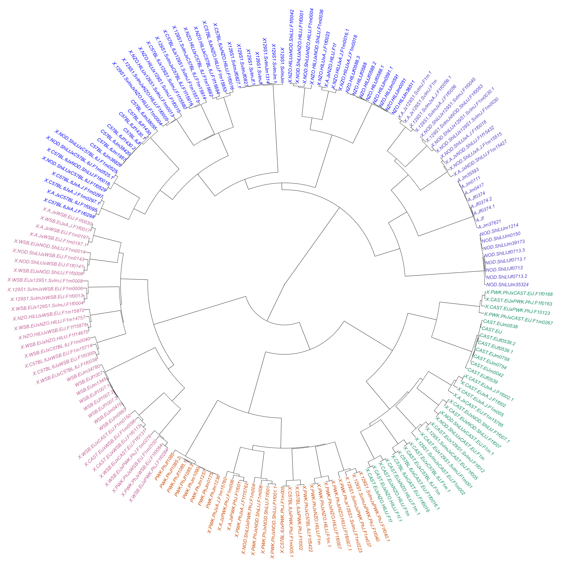
| Version | Author | Date |
|---|---|---|
| 3501596 | sam-widmayer | 2022-11-09 |
From here we curated a set of genotypes for each CC/DO founder strain that were fixed across replicate samples from that strain.
# Loop creates a data frame of consensus genotype calls for each CC/DO founder strain
# In this case, "consensus" is designated by all samples of the same strain having identical genotype calls for the same marker
founder_palette <- qtl2::CCcolors
names(founder_palette) <- founder_strains
founder_palette_2 <- founder_palette
names(founder_palette_2) <- gsub(names(founder_palette_2),pattern = "[.]", replacement = "/")
for(f in founder_strains){

  print(paste("Generating Calls for",f))

  # Pulling the samples and genotypes for each CC/DO founder strain
  founder.geno.array <- all_founder_samples %>%
    dplyr::filter(dam == f,
                  sire == f) %>%
    # Attach all genotypes
    dplyr::left_join(.,genos.flagged, by = "sample") %>%
    # Use only high-quality markers
    dplyr::filter(marker_flag != "FLAG")


  # Count the number of unique allele calls for each marker
  founder.allele.counts <- founder.geno.array %>%
    dplyr::group_by(marker, genotype) %>%
    dplyr::count()

  # Collect markers which have identical genotypes across samples from the same founder
  complete_founder_genos <- founder.allele.counts %>%
    dplyr::filter(n == max(founder.allele.counts$n)) %>%
    dplyr::select(-n) %>%
    `colnames<-`(c("marker",f))

  # Collect markers where there is some disagreement
  incomplete_founder_genos <- founder.allele.counts %>%
    dplyr::filter(n != max(founder.allele.counts$n)) %>%
    dplyr::select(-n) %>%
    `colnames<-`(c("marker",f))

  # Filter sample genotypes to markers with genotype disagreement
  incomplete_founder_genos_samples <- founder.geno.array %>%
    dplyr::filter(marker %in% unique(incomplete_founder_genos$marker)) %>%
    dplyr::select(sample, genotype, marker) %>%
    dplyr::arrange(marker)

  # Join intensities to discordant genotyped samples
  incomplete_founder_genos_ints_samples <- long_intensities[,c(1,2,3,6)] %>%
    dplyr::right_join(.,incomplete_founder_genos_samples) %>%
    dplyr::left_join(., mm_metadata %>% dplyr::select(marker, chr))

  # Create nested list by marker of sample genotypes and respective intensities to be able to eliminate certain genotypes off the bat based on outlier intensity values *within* a founder background
  incomplete_founder_genos_ints_samples_nested <- incomplete_founder_genos_ints_samples %>%
    dplyr::group_by(marker) %>%
    tidyr::nest()

  # Remove samples with extreme intensity values to try to create better consensus for the founder strain
  incomplete_founder_consensus <- purrr::pmap(.l = list(incomplete_founder_genos_ints_samples_nested$marker,
                                                        incomplete_founder_genos_ints_samples_nested$data,
                                                        rep(f, length(incomplete_founder_genos_ints_samples_nested$data))),
                                              .f = removeExtremeInts) %>%
    Reduce(rbind,.)

  # Identify markers where there is now 1 genotype across samples after removing extreme intensities
  recaptured_tally <- incomplete_founder_consensus %>%
    dplyr::group_by(marker) %>%
    dplyr::count() %>%
    dplyr::filter(n == 1)

  # Re-attach these re-inferred genotype calls to the consensus that already exists
  founder_genos <- complete_founder_genos %>%
    dplyr::bind_rows(.,incomplete_founder_consensus %>%
                       dplyr::filter(marker %in% recaptured_tally$marker))

  # Assign these calls to a founder object
  assign(paste0("Calls_",f), founder_genos)

}
[1] "Generating Calls for A.J"
[1] "Generating Calls for C57BL.6J"
[1] "Generating Calls for 129S1.SvImJ"
[1] "Generating Calls for NOD.ShiLtJ"
[1] "Generating Calls for NZO.HILtJ"
[1] "Generating Calls for CAST.EiJ"
[1] "Generating Calls for PWK.PhJ"
[1] "Generating Calls for WSB.EiJ"The genotypes for intersecting markers between two strains were combined (“crossed”) to form predicted genotypes for each F1 hybrid of CC/DO founders. Then, the genotypes of each CC/DO founder F1 hybrid were compared directly to what was predicted, and the concordance shown below is the proportion of markers of each individual that match this prediction.
# Build a list of founder consensus genotypes for good markers
founder_consensus_calls <- list(Calls_A.J, Calls_C57BL.6J, Calls_129S1.SvImJ, Calls_NOD.ShiLtJ,
                                Calls_NZO.HILtJ, Calls_CAST.EiJ, Calls_PWK.PhJ, Calls_WSB.EiJ)

# Generate a data frame with good markers as the sole column
good_markers <- genos.flagged %>%
  dplyr::distinct(marker, marker_flag) %>%
  dplyr::filter(marker_flag != "FLAG")

# Loop through the exisitng consensus calls and filter down to good markers
filtered_consensus_calls <- purrr::map(founder_consensus_calls,
                                       function(x){
                                         x %>%
                                           dplyr::filter(marker %in% good_markers$marker)
                                         }) %>%
  Reduce(full_join, .)
# Replace "." in strain names with "/"
colnames(filtered_consensus_calls)[-1] <- gsub(colnames(filtered_consensus_calls)[-1], pattern = "[.]", replacement = "/")


# Filter samples down to inbred strains and attach a proper strain name column
founder_sample_metadata <- all_founder_samples %>%
  dplyr::mutate(strain = if_else(dam == sire, true = dam, false = "CROSS")) %>%
  dplyr::filter(bg == "INBRED",
                strain %in% founder_strains) %>%
  dplyr::mutate(strain = gsub(strain,pattern = "[.]", replacement = "/"))
#   sample     dam   sire  bad_sample inferred.sex resexed bg     founder weird.founder strain
#   <chr>      <chr> <chr> <chr>      <chr>        <lgl>   <chr>  <chr>   <chr>         <chr>
# 1 A.Jf       A.J   A.J   ""         f            FALSE   INBRED FOUNDER ""            A/J
# 2 A.Jf0374   A.J   A.J   ""         f            FALSE   INBRED FOUNDER ""            A/J
# 3 A.Jf0374.1 A.J   A.J   ""         f            FALSE   INBRED FOUNDER ""            A/J
# 4 A.Jf0374.2 A.J   A.J   ""         f            FALSE   INBRED FOUNDER ""            A/J
# 5 A.Jm0111   A.J   A.J   ""         m            FALSE   INBRED FOUNDER ""            A/J
# 6 A.Jm0417   A.J   A.J   ""         m            FALSE   INBRED FOUNDER ""            A/J


# Create column index for intensity data tables
founder_samples_for_ints <- c("marker",founder_sample_metadata$sample)
founder_x_int <- x_intensities[marker %in% good_markers$marker,..founder_samples_for_ints] %>%
  tidyr::pivot_longer(-marker, names_to = "sample", values_to = "x_int") %>%
  dplyr::left_join(., founder_sample_metadata, by = "sample")
founder_y_int <- y_intensities[marker %in% good_markers$marker,..founder_samples_for_ints] %>%
  tidyr::pivot_longer(-marker, names_to = "sample", values_to = "y_int") %>%
  dplyr::left_join(., founder_sample_metadata, by = "sample")

# Identify consensus calls that have complete data across founders
founder_consensus_complete <- filtered_consensus_calls[complete.cases(filtered_consensus_calls),]
# Identify consensus calls that have DO NOT have complete data across founders (i.e. maybe some sort of discrepancy among samples contributing to that founder)
founder_consensus_incomplete <- filtered_consensus_calls[!complete.cases(filtered_consensus_calls),]

# Attach intensity data to sample genotypes and nest the data for QCing in next step
missing_consensus_calls_nested <- founder_consensus_incomplete %>%
  tidyr::pivot_longer(-marker, names_to = "strain", values_to = "genotype") %>%
  dplyr::full_join(., founder_x_int %>%
                     dplyr::filter(marker %in% founder_consensus_incomplete$marker) %>%
                     dplyr::select(marker, sample, strain, x_int)) %>%
  dplyr::full_join(.,founder_y_int %>%
                     dplyr::filter(marker %in% founder_consensus_incomplete$marker) %>%
                     dplyr::select(marker, sample, strain, y_int)) %>%
  dplyr::rename(consensus_genotype = genotype) %>%
  dplyr::left_join(., genos.flagged %>%
                     dplyr::filter(marker_flag != "FLAG",
                                  marker %in% founder_consensus_incomplete$marker) %>%
                     dplyr::select(marker, sample, genotype) %>%
                     dplyr::rename(sample_genotype = genotype)) %>%
  dplyr::ungroup() %>%
  dplyr::group_by(marker) %>%
  tidyr::nest()
In order to generate a consensus call for each CC/DO founder, we had to determine whether individual samples for a given founder were correctly typed and, if the marker failed, eliminate it so that consensus could be formed. Below is an example of what that might look like for an individual marker. Note how when at least one sample for a given strain is not assigned one of the two expected alleles, the consensus is an “NA”.
# Sample a marker at random
m <- sample(seq(1:length(missing_consensus_calls_nested$marker)), size = 1)
sample_genotypes_plot <- ggplot() +
  geom_point(data = missing_consensus_calls_nested$data[[m]], mapping = aes(x = x_int,
                                             y = y_int,
                                             colour = sample_genotype,
                                             label = sample)) +
  scale_colour_manual(values = brewer.pal(4,"Set2")) +
  QCtheme +
  ggtitle(paste0("Sample genotypes for marker", missing_consensus_calls_nested$marker[[m]]))
Warning in geom_point(data = missing_consensus_calls_nested$data[[m]], mapping =
aes(x = x_int, : Ignoring unknown aesthetics: labelconsensus_genotypes_plot <- ggplot() +
geom_point(data = missing_consensus_calls_nested$data[[m]], mapping = aes(x = x_int,
y = y_int,
colour = consensus_genotype,
label = sample)) +
scale_colour_manual(values = brewer.pal(4,"Set1")) +
QCtheme +
ggtitle(paste0("Resulting consensus genotypes for marker ", missing_consensus_calls_nested$marker[[m]]))Warning in geom_point(data = missing_consensus_calls_nested$data[[m]], mapping =
aes(x = x_int, : Ignoring unknown aesthetics: labelggplotly(sample_genotypes_plot)ggplotly(consensus_genotypes_plot)We observed 1847 markers without a consensus genotype for at least one strain. For each one, we used the intensity data to identify problematic founder samples, eliminate them, and then use good founder samples to re-classify missing consensus genotypes for strains where they were missing before. Below is the expected output of that process.
example_output <- findConsensusGenotypes(mk = missing_consensus_calls_nested$marker[[m]],
                                         data =  missing_consensus_calls_nested$data[[m]])
recoded_consensus_genotypes_plot <- ggplot() +
  geom_point(data = example_output[[3]], mapping = aes(x = x_int,
                                                       y = y_int,
                                                       colour = consensus_genotype,
                                                       fill = recoded,
                                                       label = sample), shape = 21) +
  scale_fill_manual(values = c("black","white")) +
  scale_colour_manual(values = brewer.pal(4,"Set1")) +
  QCtheme +
  ggtitle(paste0("Re-coded consensus genotypes for marker", missing_consensus_calls_nested$marker[[m]]))
Warning in geom_point(data = example_output[[3]], mapping = aes(x = x_int, :
Ignoring unknown aesthetics: labelggplotly(recoded_consensus_genotypes_plot)# Loop through markers where at least one strain lacked a consensus call and re-assign using other founder sample genotype data
founder_consensus_incomplete_recoded <- suppressWarnings(furrr::future_map2(missing_consensus_calls_nested$marker,
missing_consensus_calls_nested$data,
findConsensusGenotypes))
founder_consensus_incomplete_recoded_tr <- purrr::transpose(founder_consensus_incomplete_recoded)
new_consensus_founders <- Reduce(dplyr::bind_rows,founder_consensus_incomplete_recoded_tr[[1]])
updated_founder_sample_genotypes <- Reduce(dplyr::bind_rows,founder_consensus_incomplete_recoded_tr[[2]])
# Update original consensus calls with re-assigned consensus calls
clean_founder_consensus_genotypes <- founder_consensus_complete %>%
dplyr::bind_rows(.,new_consensus_founders)By using probe intensities and replicate samples among founder strains to re-evaluate consensus genotype calls, we recovered genotypes for 69.5722794% of those for which consensus genotypes were previously missing. Finally, we quantified the concordance between all founder sample genotypes (including samples from crosses between founders) and those predicted based on the updated consensus genotype calls.
# Assemble a list of predicted genotypes for F1s by combining each founder-specific dataframe of calls
founder_strains_2 <- gsub(founder_strains, pattern = "[.]", replacement =  "/")
for(f in founder_strains_2){
  clean_founder_con <- clean_founder_consensus_genotypes %>%
    dplyr::ungroup() %>%
    dplyr::select(marker, f)
  assign(paste0("Clean_Calls_",f), clean_founder_con)
}
Warning: Using an external vector in selections was deprecated in tidyselect 1.1.0.
ℹ Please use `all_of()` or `any_of()` instead.
# Was:
data %>% select(f)
# Now:
data %>% select(all_of(f))
See <https://tidyselect.r-lib.org/reference/faq-external-vector.html>.# First form a list of dams that comprise each F1 cross type
dams <- data.frame(tidyr::expand_grid(founder_strains_2, founder_strains_2, .name_repair = "minimal")) %>%
`colnames<-`(c("dams","sires")) %>%
# Select crosses between strains
# filter(dams != sires) %>%
dplyr::select(dams) %>%
as.list()
# Loop through the list of cross types and pull in genotype call objects
dam_calls <- list()
for(i in 1:length(dams$dams)){
dam_calls[[i]] <- get(ls(pattern = paste0("Clean_Calls_",dams$dams[i])))
}
# Do the same for the sires for each F1
sires <- data.frame(tidyr::expand_grid(founder_strains_2, founder_strains_2, .name_repair = "minimal")) %>%
`colnames<-`(c("dams","sires")) %>%
# filter(dams != sires) %>%
dplyr::select(sires) %>%
as.list()
sire_calls <- list()
for(i in 1:length(sires$sires)){
sire_calls[[i]] <- get(ls(pattern = paste0("Clean_Calls_",sires$sires[i])))
}
# Compare the predicted genotypes (from consensus calls) to the actual genotypes of each sample
# founder_background_QC(dam = dam_calls[[6]], sire = sire_calls[[6]])
bg_QC <- purrr::map2(dam_calls, sire_calls, founder_background_QC)[1] "Running QC: A.J"
[1] "Running QC: (A.JxC57BL.6J)F1"
[1] "Running QC: (A.Jx129S1.SvImJ)F1"
[1] "Running QC: (A.JxNOD.ShiLtJ)F1"
[1] "Running QC: (A.JxNZO.HILtJ)F1"
[1] "Running QC: (A.JxCAST.EiJ)F1"
[1] "Running QC: (A.JxPWK.PhJ)F1"
[1] "Running QC: (A.JxWSB.EiJ)F1"
[1] "Running QC: (C57BL.6JxA.J)F1"
[1] "Running QC: C57BL.6J"
[1] "Running QC: (C57BL.6Jx129S1.SvImJ)F1"
[1] "Running QC: (C57BL.6JxNOD.ShiLtJ)F1"
[1] "Running QC: (C57BL.6JxNZO.HILtJ)F1"
[1] "Running QC: (C57BL.6JxCAST.EiJ)F1"
[1] "Running QC: (C57BL.6JxPWK.PhJ)F1"
[1] "Running QC: (C57BL.6JxWSB.EiJ)F1"
[1] "Running QC: (129S1.SvImJxA.J)F1"
[1] "Running QC: (129S1.SvImJxC57BL.6J)F1"
[1] "Running QC: 129S1.SvImJ"
[1] "Running QC: (129S1.SvImJxNOD.ShiLtJ)F1"
[1] "Running QC: (129S1.SvImJxNZO.HILtJ)F1"
[1] "Running QC: (129S1.SvImJxCAST.EiJ)F1"
[1] "Running QC: (129S1.SvImJxPWK.PhJ)F1"
[1] "Running QC: (129S1.SvImJxWSB.EiJ)F1"
[1] "Running QC: (NOD.ShiLtJxA.J)F1"
[1] "Running QC: (NOD.ShiLtJxC57BL.6J)F1"
[1] "Running QC: (NOD.ShiLtJx129S1.SvImJ)F1"
[1] "Running QC: NOD.ShiLtJ"
[1] "Running QC: (NOD.ShiLtJxNZO.HILtJ)F1"
[1] "Running QC: (NOD.ShiLtJxCAST.EiJ)F1"
[1] "Running QC: (NOD.ShiLtJxPWK.PhJ)F1"
[1] "Running QC: (NOD.ShiLtJxWSB.EiJ)F1"
[1] "Running QC: (NZO.HILtJxA.J)F1"
[1] "Running QC: (NZO.HILtJxC57BL.6J)F1"
[1] "Running QC: (NZO.HILtJx129S1.SvImJ)F1"
[1] "Running QC: (NZO.HILtJxNOD.ShiLtJ)F1"
[1] "Running QC: NZO.HILtJ"
[1] "Running QC: (NZO.HILtJxCAST.EiJ)F1"
[1] "Running QC: (NZO.HILtJxPWK.PhJ)F1"
[1] "Running QC: (NZO.HILtJxWSB.EiJ)F1"
[1] "Running QC: (CAST.EiJxA.J)F1"
[1] "Running QC: (CAST.EiJxC57BL.6J)F1"
[1] "Running QC: (CAST.EiJx129S1.SvImJ)F1"
[1] "Running QC: (CAST.EiJxNOD.ShiLtJ)F1"
[1] "Running QC: (CAST.EiJxNZO.HILtJ)F1"
[1] "Running QC: CAST.EiJ"
[1] "Running QC: (CAST.EiJxPWK.PhJ)F1"
[1] "Running QC: (CAST.EiJxWSB.EiJ)F1"
[1] "Running QC: (PWK.PhJxA.J)F1"
[1] "Running QC: (PWK.PhJxC57BL.6J)F1"
[1] "Running QC: (PWK.PhJx129S1.SvImJ)F1"
[1] "Running QC: (PWK.PhJxNOD.ShiLtJ)F1"
[1] "Running QC: (PWK.PhJxNZO.HILtJ)F1"
[1] "Running QC: (PWK.PhJxCAST.EiJ)F1"
[1] "Running QC: PWK.PhJ"
[1] "Running QC: (PWK.PhJxWSB.EiJ)F1"
[1] "Running QC: (WSB.EiJxA.J)F1"
[1] "Running QC: (WSB.EiJxC57BL.6J)F1"
[1] "Running QC: (WSB.EiJx129S1.SvImJ)F1"
[1] "Running QC: (WSB.EiJxNOD.ShiLtJ)F1"
[1] "Running QC: (WSB.EiJxNZO.HILtJ)F1"
[1] "Running QC: (WSB.EiJxCAST.EiJ)F1"
[1] "Running QC: (WSB.EiJxPWK.PhJ)F1"
[1] "Running QC: WSB.EiJ"# Keep outputs from the QC that are lists; if QC wasn't performed for a given background, the output was a character vector warning
founder_background_QC_tr <- bg_QC %>%
purrr::keep(., is.list) %>%
# Instead of having 64 elements of lists of two, have two lists of 64:
# 1) All good genotypes from each cross with concordance values
# 2) All concordance summaries for each cross
purrr::transpose(.)
# Bind together all concordance summaries
founder_concordance_df <- Reduce(rbind, founder_background_QC_tr[[2]])
# If all markers for a given chromosome type were either concordant or discordant, NAs are returned
# This step assigns those NA values a 0
founder_concordance_df[is.na(founder_concordance_df)] <- 0
# Form concordance as a percentage
founder_concordance_df_2 <- founder_concordance_df %>%
dplyr::mutate(concordance = MATCH/(MATCH + `NO MATCH`)) %>%
dplyr::mutate(dam = gsub(dam, pattern = "[.]", replacement = "/"),
sire = gsub(sire, pattern = "[.]", replacement = "/"))
founder_concordance_df_2$alt_chr <- factor(founder_concordance_df_2$alt_chr,
levels = c("Autosome","X","Y","M","Other"))
founder_concordance_df_3 <- founder_concordance_df_2 %>%
dplyr::filter(alt_chr == "Autosome")
concordance_plot <- ggplot(founder_concordance_df_3, mapping = aes(x = dam, y = concordance, color = dam, fill = sire)) +
geom_jitter(shape = 21, width = 0.25) +
scale_fill_manual(values = founder_palette_2) +
scale_colour_manual(values = founder_palette_2) +
ylim(c(0.5,1.05)) +
labs(x = "Dam Founder Strain",
y = "Autosomal Genotype Concordance") +
QCtheme
ggplotly(concordance_plot)Writing reference files
The list of output file types following QC is as follows:
Genotype file; rows = markers, columns = samples
Probe intensity file; rows = markers, columns = samples
Sample metadata; columns = sample, strain, sex
Each file type is generated for:
All good samples
Eight CC/DO founder strains
In total, 75058 markers and 353 samples passed the QC steps we imposed, and wrote these genotype data and metadata to new reference files.
# Generate genotype files for all good samples and all good markers
reference_genos_all_samples <- control_genotypes[marker %in% good_markers$marker,..good_samples]

founder_sample_names <- c("marker",unique(founder_concordance_df_3$sample))

reference_genos_founder_samples <- reference_genos_all_samples[,..founder_sample_names]
reference_genos_founder_samples_complete <- reference_genos_founder_samples[!marker %in% updated_founder_sample_genotypes$marker,]
reference_genos_founder_samples_updated <- reference_genos_founder_samples_complete %>%
  dplyr::bind_rows(., updated_founder_sample_genotypes[which(updated_founder_sample_genotypes$marker %in% reference_genos_founder_samples$marker),])
nonfounder_samples <- c("marker",colnames(reference_genos_all_samples)[!colnames(reference_genos_all_samples) %in% founder_sample_names])
reference_genos_nonfounder_samples <- reference_genos_all_samples[,..nonfounder_samples]
pre_final_reference_genos <- reference_genos_nonfounder_samples %>%
  dplyr::full_join(., reference_genos_founder_samples_updated)

final_reference_genos <- pre_final_reference_genos[, lapply(.SD, function(x) replace(x, which(is.na(x)), "N"))]
reference_genos_founders_final <- final_reference_genos[,..founder_sample_names]


# Intensities
reference_xints_all_samples <- x_intensities[marker %in% good_markers$marker,..good_samples]
reference_yints_all_samples <- y_intensities[marker %in% good_markers$marker,..good_samples]

founder_mean_x_ints <- founder_x_int %>%
  dplyr::left_join(.,mm_metadata %>%
                     dplyr::select(marker, chr), by = "marker") %>%
  dplyr::select(marker, chr, sample, strain, inferred.sex, x_int) %>%
  dplyr::group_by(marker, strain) %>%
  dplyr::summarise(x_int = mean(x_int)) %>%
  tidyr::pivot_wider(names_from = strain, values_from = x_int) %>%
  dplyr::filter(marker %in% good_markers$marker)

founder_mean_y_ints <- founder_y_int %>%
  dplyr::left_join(.,mm_metadata %>%
                     dplyr::select(marker, chr), by = "marker") %>%
  dplyr::select(marker, chr, sample, strain, inferred.sex, y_int) %>%
  dplyr::group_by(marker, strain) %>%
  dplyr::summarise(y_int = mean(y_int)) %>%
  tidyr::pivot_wider(names_from = strain, values_from = y_int)%>%
  dplyr::filter(marker %in% good_markers$marker)

final_founder_consensus_genotypes <- clean_founder_consensus_genotypes %>%
  dplyr::filter(marker %in% good_markers$marker)
final_founder_consensus_genotypes[is.na(final_founder_consensus_genotypes)] <- "N"

# All sample metadata
pre_metadata <- sample.meta %>%
  dplyr::select(sample, inferred.sex, resexed) %>%
  dplyr::mutate(bad_sample = if_else(sample %in% bad_samples, true = "BAD SAMPLE", false = "")) %>%
  dplyr::rename(sex = inferred.sex)

strain_assignment <- all_founder_samples %>%
  dplyr::ungroup() %>%
  dplyr::distinct(sample, dam, sire) %>%
  dplyr::mutate(strain = if_else(dam == sire,
                                 true = dam,
                                 false = paste0("(",dam,"x",sire,")F1"))) %>%
  dplyr::left_join(pre_metadata,.) %>%
  dplyr::select(sample, sex, resexed, strain)
unassigned_strains <- strain_assignment %>%
  dplyr::filter(is.na(strain))
new_strains <- purrr::map(unassigned_strains$sample, findStrain) %>%
  unlist()
unassigned_strains$strain <- new_strains
remaining_nonfounder_samples <- unassigned_strains %>%
  dplyr::mutate(mouse.id.1 = stringr::str_sub(strain, -1),
                strain = dplyr::if_else(mouse.id.1 %in% c("m","f"),
                                        true = str_sub(string = strain, 1, nchar(strain)-1),
                                        false = strain)) %>%
  dplyr::select(-mouse.id.1) %>%
  dplyr::mutate(strain = dplyr::case_when(strain %in% c("FVB.M","FVB.M.1","FVB.M.2","FVB") ~ "FVB.NJ",
                                          strain %in% c("KOMP.cell.DNA.JM8.1","KOMP.cell.DNA.JM8.2") ~ "KOMP.cell.DNA.JM8",
                                          strain == "PWD" ~ "PWD.PhJ",
                                          strain == "X129S1.Svl" ~ "X129S1.SvlmJ",
                                          TRUE ~ strain),
                strain = dplyr::if_else(str_sub(strain, 1, 2) == "X1",
                                        true = str_sub(strain, 2),
                                        false = strain),
                strain = dplyr::if_else(str_sub(strain, 1, 2) == "X.",
                                        true = str_sub(strain, 3),
                                        false = strain),
                strain = dplyr::if_else(str_detect(strain, "F1") == TRUE,
                                        true = paste0("(",gsub(strain, pattern = ".F1", replacement = ")F1")),
                                        false = strain))
reference_sample_metadata <- strain_assignment %>%
  dplyr::filter(!is.na(strain)) %>%
  dplyr::bind_rows(.,remaining_nonfounder_samples) %>%
  dplyr::mutate(strain = gsub(strain, pattern = "[.]", replacement = "/"),
                strain = dplyr::case_when(strain == "BTBR/T///tf/J" ~ "BTBR T<+>tf/J",
                                          strain == "H3f3aSA/Neo/GFP/fl//" ~ "H3f3aSA-Neo-GFP-fl/+",
                                          strain == "H3f3bSA/Neo/tdTo" ~ "H3f3bSA-Neo-tdTomato-fl/SA-Neo-tdTomato-fl",
                                          strain == "KOMP/cell/DNA/JM8" ~ "KOMP cell DNA JM8",
                                          strain == "Oct4/GFP/CreERT2Tg/Tg" ~ "Oct4-GFP-CreERT2Tg/Tg",
                                          strain == "Sox2/CreTg//Tg/" ~ "Sox2-CreTg/(Tg)",
                                          strain == "Tgln/////Cre/" ~ "Tgln -/- Cre+",
                                          strain == "Nestin/////Cre/" ~ "Nestin -/- Cre+",
                                          TRUE ~ strain))

founder_sample_metadata_conc <- founder_concordance_df_3 %>%
  dplyr::left_join(., reference_sample_metadata) %>%
  dplyr::ungroup() %>%
  dplyr::select(sample, strain, sex, dam, sire, concordance) %>%
  dplyr::mutate(dam = case_when(dam == "A/J" ~ "A",
                                dam == "C57BL/6J" ~ "B",
                                dam == "129S1/SvImJ" ~ "C",
                                dam == "NOD/ShiLtJ" ~ "D",
                                dam == "NZO/HILtJ" ~ "E",
                                dam == "CAST/EiJ" ~ "F",
                                dam == "PWK/PhJ" ~ "G",
                                dam == "WSB/EiJ" ~ "H"),
                sire = case_when(sire == "A/J" ~ "A",
                                sire == "C57BL/6J" ~ "B",
                                sire == "129S1/SvImJ" ~ "C",
                                sire == "NOD/ShiLtJ" ~ "D",
                                sire == "NZO/HILtJ" ~ "E",
                                sire == "CAST/EiJ" ~ "F",
                                sire == "PWK/PhJ" ~ "G",
                                sire == "WSB/EiJ" ~ "H")) %>%
  tidyr::unite("letter", dam:sire, sep = "")


dir.create("output", showWarnings = F)
dir.create("output/MegaMUGA", showWarnings = F)


  write.csv(reference_genos_all_samples,
            file = "output/MegaMUGA/MegaMUGA_genotypes.csv",
            row.names = F)
  system("gzip output/MegaMUGA/MegaMUGA_genotypes.csv")


  write.csv(reference_xints_all_samples,
            file = "output/MegaMUGA/MegaMUGA_x_intensities.csv",
            row.names = F)
  system("gzip output/MegaMUGA/MegaMUGA_x_intensities.csv")


  write.csv(reference_yints_all_samples,
            file = "output/MegaMUGA/MegaMUGA_y_intensities.csv",
            row.names = F)
  system("gzip output/MegaMUGA/MegaMUGA_y_intensities.csv")


  write.csv(reference_sample_metadata,
            file = "output/MegaMUGA/MegaMUGA_sample_metadata.csv",
            row.names = F)


  write.csv(final_founder_consensus_genotypes,
            file = "output/MegaMUGA/MegaMUGA_founder_consensus_genotypes.csv",
            row.names = F)
  system("gzip output/MegaMUGA/MegaMUGA_founder_consensus_genotypes.csv")


  write.csv(founder_mean_x_ints,
            file = "output/MegaMUGA/MegaMUGA_founder_mean_x_intensities.csv",
            row.names = F)
  system("gzip output/MegaMUGA/MegaMUGA_founder_mean_x_intensities.csv")


  write.csv(founder_mean_y_ints,
            file = "output/MegaMUGA/MegaMUGA_founder_mean_y_intensities.csv",
            row.names = F)
  system("gzip output/MegaMUGA/MegaMUGA_founder_mean_y_intensities.csv")


  write.csv(founder_sample_metadata_conc,
            file = "output/MegaMUGA/MegaMUGA_founder_metadata.csv",
            row.names = F)
sessionInfo()R version 4.2.1 (2022-06-23)
Platform: x86_64-apple-darwin17.0 (64-bit)
Running under: macOS Big Sur ... 10.16
Matrix products: default
BLAS: /Library/Frameworks/R.framework/Versions/4.2/Resources/lib/libRblas.0.dylib
LAPACK: /Library/Frameworks/R.framework/Versions/4.2/Resources/lib/libRlapack.dylib
locale:
[1] en_US.UTF-8/en_US.UTF-8/en_US.UTF-8/C/en_US.UTF-8/en_US.UTF-8
attached base packages:
[1] stats graphics grDevices utils datasets methods base
other attached packages:
[1] RColorBrewer_1.1-3 ape_5.6-2 progress_1.2.2 plotly_4.10.1
[5] ggplot2_3.4.0 DT_0.26 magrittr_2.0.3 qtl2_0.28
[9] furrr_0.3.1 future_1.29.0 purrr_0.3.5 data.table_1.14.4
[13] stringr_1.4.1 tidyr_1.2.1 dplyr_1.0.10
loaded via a namespace (and not attached):
[1] httr_1.4.4 sass_0.4.2 bit64_4.0.5 jsonlite_1.8.3
[5] viridisLite_0.4.1 bslib_0.4.1 assertthat_0.2.1 highr_0.9
[9] blob_1.2.3 yaml_2.3.6 globals_0.16.1 pillar_1.8.1
[13] RSQLite_2.2.18 lattice_0.20-45 glue_1.6.2 digest_0.6.30
[17] promises_1.2.0.1 colorspace_2.0-3 htmltools_0.5.3 httpuv_1.6.6
[21] pkgconfig_2.0.3 listenv_0.8.0 scales_1.2.1 whisker_0.4
[25] later_1.3.0 git2r_0.30.1 tibble_3.1.8 generics_0.1.3
[29] farver_2.1.1 ellipsis_0.3.2 cachem_1.0.6 withr_2.5.0
[33] lazyeval_0.2.2 cli_3.4.1 crayon_1.5.2 memoise_2.0.1
[37] evaluate_0.18 fs_1.5.2 fansi_1.0.3 parallelly_1.32.1
[41] nlme_3.1-157 tools_4.2.1 prettyunits_1.1.1 hms_1.1.2
[45] lifecycle_1.0.3 munsell_0.5.0 compiler_4.2.1 jquerylib_0.1.4
[49] rlang_1.0.6 grid_4.2.1 rstudioapi_0.14 htmlwidgets_1.5.4
[53] crosstalk_1.2.0 labeling_0.4.2 rmarkdown_2.18 gtable_0.3.1
[57] codetools_0.2-18 DBI_1.1.3 R6_2.5.1 knitr_1.40
[61] fastmap_1.1.0 bit_4.0.4 utf8_1.2.2 workflowr_1.7.0
[65] rprojroot_2.0.3 stringi_1.7.8 parallel_4.2.1 Rcpp_1.0.9
[69] vctrs_0.5.0 tidyselect_1.2.0 xfun_0.34